-
October 17, 2025
Single-button reproducibility: The what, the why, and the how
One of the initial visions for computational reproducibility dates back to the early 90s, where Claerbout and Karrenbach imagined researchers able to reproduce their results “a year or more later with a single button.” In other words, they hoped it would be possible to run a single command to transform any study’s raw data into figures, tables, and finally a complete research article. We never quite got there, but we could, and we should.
flowchart LR
    A[Collect data] --> B[Process data]
    B --> C[Visualize data]
    C --> D[Compile paper]

    style A fill:#90EE90
    style B fill:#87CEEB
    style C fill:#87CEEB
    style D fill:#87CEEB
These days, the open science movement has made code and data sharing more appreciated and more common, which is a great achievement, but often what is shared—sometimes called a “repro pack”—is not single-button reproducible. In fact, in most cases what’s shared is not reproducible at all, hence why it’s called a reproducibility crisis.
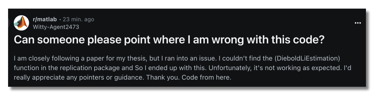
Download a random repro pack from Figshare or Zenodo and if you’re lucky you’ll find a README with a list of manual steps explaining how to install necessary packages, download data to specific locations, and run the project’s analyses and visualizations. Often you’ll see a collection of numbered scripts and/or notebooks with no instructions at all. Sometimes you’ll need to manually modify the code to run on your system because the original author used absolute paths or it depends on credentials for some external web service. In other words, these are not even close to being single-button reproducible.
To be clear, this level of transparency and willingness to share messy code is admirable and should be rewarded. Fragility in evidence generation does not necessarily indicate incorrect conclusions, laziness, or misconduct. Nevertheless, that fragility and the lack of automation in research workflows present a huge opportunity to benefit both the community and the individuals involved.
Benefits to the community
It’s not hard to imagine why it would be helpful for every study to ship with a single-button repro pack. If we think of each new one building upon the last like floors of a skyscraper, spending time and effort to get a predecessor’s code running is like having to rebuild part of the floor below, which is clearly inefficient. Yet this is the story for many grad students and postdocs. In this example, getting software from a previous student back to a runnable state took half a year. Imagine if that time were spent creating new things rather than reproducing old ones to get back to square one, and then imagine scaling those gains across all researchers.

When you ship a single-button reproducible project with your paper others can build on top of it and the whole building (our collective knowledge) gets built more quickly. Even if the code isn’t nicely generalized and modularized, i.e., it’s a collection of highly specific scripts and notebooks rather than a software product like an application or library, it’s still much more useful to have something that works than something that does not. With a working project, one can take small steps to evolve it towards doing something new. A working project is worth studying and learning from.
With a non-working project, it can be challenging to even know where to start, and many will choose to start from scratch. Furthermore, it’s a lot easier to productize an algorithm when you have a working reference implementation, even if it’s going to be rewritten. Personally, I’d much rather start with a functioning and well-orchestrated collection of one-off scripts than a half-baked general purpose tool, even if the latter is thoroughly documented.
Imagine if this student didn't need to waste their time reverse engineering a non-working repro pack. 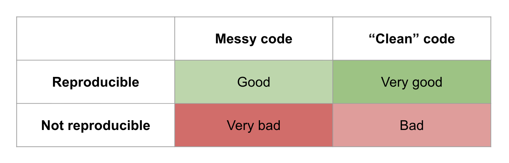
Messy code that runs is better than 'clean' code that doesn't. Benefits to the individual
Shipping single-button reproducible projects will surely benefit those looking to build on the work, but what about the original authors themselves? If we want them to play along they’re going to need to get something out of it, and for most this is going to mean things that tenure committees and funding organizations care about like publications and citations. There’s evidence that working openly attracts more citations, and here I’ll argue that automation will also achieve faster time-to-publication with improved quality.
In software engineering it’s well known that build, test, and deployment pipelines are worth automating because automation reduces waste and eliminates pain points, ultimately allowing for faster and more frequent iterations. With more iterations—more times at bat—comes a higher quality product and more positive impact on customers and the business. Fully-automated workflows are much less common in science, but the value comes from the same principles.
Consider a workflow like the one below. It involves installing dependencies, downloading data, running scripts in different languages, running notebooks, saving and uploading figures to a writing tool like Overleaf, and then finally exporting a PDF to share with the world. When not automated, each line connecting the boxes represents “computational logistics,” which take time and don’t add value to the final product. If any of these steps needs to be done more than once (which is almost guaranteed), their automation would speed up time-to-publication.
flowchart LR
    A[Install Python packages] --> B[Run Python script 1]
    AA[Download data] --> B
    B --> C[Run notebook 1]
    C --> D[Edit figure 1 in Photoshop]
    D --> E[Upload figure 1 to Overleaf]
    E --> F[Export PDF]
    G[Run Python script 2] --> C
    A --> G

    H[Install R packages] --> I[Run R script 1]
    G --> I
    I --> J[Run notebook 2]
    J --> L[Upload figure 2 to Overleaf]
    L --> F

    style A fill:#87CEEB
    style AA fill:#87CEEB
    style B fill:#87CEEB
    style C fill:#87CEEB
    style D fill:#87CEEB
    style E fill:#87CEEB
    style F fill:#90EE90
    style G fill:#87CEEB
    style H fill:#87CEEB
    style I fill:#87CEEB
    style J fill:#87CEEB
    style L fill:#87CEEB
Beyond time wasted, each of these low-value-add tasks increases cognitive overhead, and switching between different apps and platforms for different tasks creates “digital tool fatigue.” Imagine we need to change something about Python script 2. Keeping track of what other steps need to be done in response is going to cost brainpower that would be better spent on so-called “Deep Work”. Scientists should be thinking up innovative ideas, not trying to remember if they need to regenerate and reupload a figure and which script created it. Again, when this process is tedious because it’s manual, there’s an inclination to do fewer iterations, which diminishes quality.
The problem with post-hoc repro packs
Sometimes you’ll take a look at a repro pack and get the feeling it was curated after the fact, not used during the work. Some journals require repro packs to be submitted and checked as part of the review process, but most of the time authors are only putting these together for the sake of doing open science. Again, this is much better than not sharing, but doing all that work at the end is another source of waste, never mind the fact it usually doesn’t result in a reproducible project. All the instructions that end up in the README—install this, run that, download here—those are the low-value-add tasks that were taking up space in the researcher’s brain the whole time. They were also making it difficult for collaborators to contribute, since likely only one person could run the entire project given how scattered around it all was.
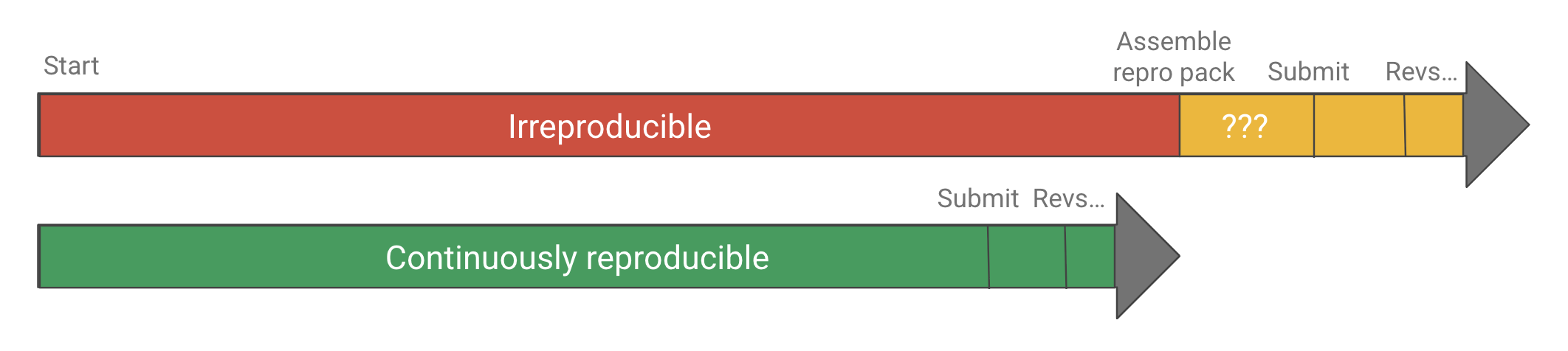
Why assemble a repro pack at the end of a project when it could be used throughout? Imagine instead that the project was automated from the start to be “continuously reproducible”, which is sometimes called practicing continuous analysis, continuous science, or continuous validation. The researcher could do some work on one aspect of the project, save it, push the button to get it into a reproducible state, and then work on the next task. They could quickly and confidently integrate changes from someone else on the team, who could run the project on their own just as easily. In addition to faster iteration cycle time, there would be no more “review anxiety,” worrying if you’ll be asked to change something, either by the principal investigator (PI), a team member, or a referee.
But what about the cost?
Let’s say you’re with me so far—you believe that there are enough iterations done and enough waste to eliminate to justify automating research project workflows end-to-end. With today’s tools and best practices, what does it take? The typical “stack” following current best practices would look something like:
- Git/GitHub for version controlling code, LaTeX input files, etc.
- Data backed up in cloud storage, Google Drive, Dropbox, etc., then archived on Figshare, Zenodo, or OSF.
- Dependencies managed with virtual environments and/or containers.
- Scripting and/or a workflow engine like Make, Snakemake, NextFlow to tie everything together and move data around when necessary.
When we ask scientists to work this way we are essentially requesting they become part-time software engineers: surveying and picking tools, designing workflows and project layouts, and writing sophisticated code to tie everything together. Some will like that and find the tools and processes exciting. Others will not. They will want to focus on the science and not want to get bogged down with what feels like a lot of extra work just to do some computation as part of their research.
In other words, today there is a very high cost to single-button reproducibility in terms of both skill and effort, and researchers are (fairly, in my opinion) perceiving that the cost is not worth the benefit, as it might even delay, not speed up time-to-publication. And so there’s the challenge. In the absence of other incentives (like punishment for irreproducible publications) we can’t expect all, or even most researchers to publish single-button reproducible projects without driving down the cost of automation.
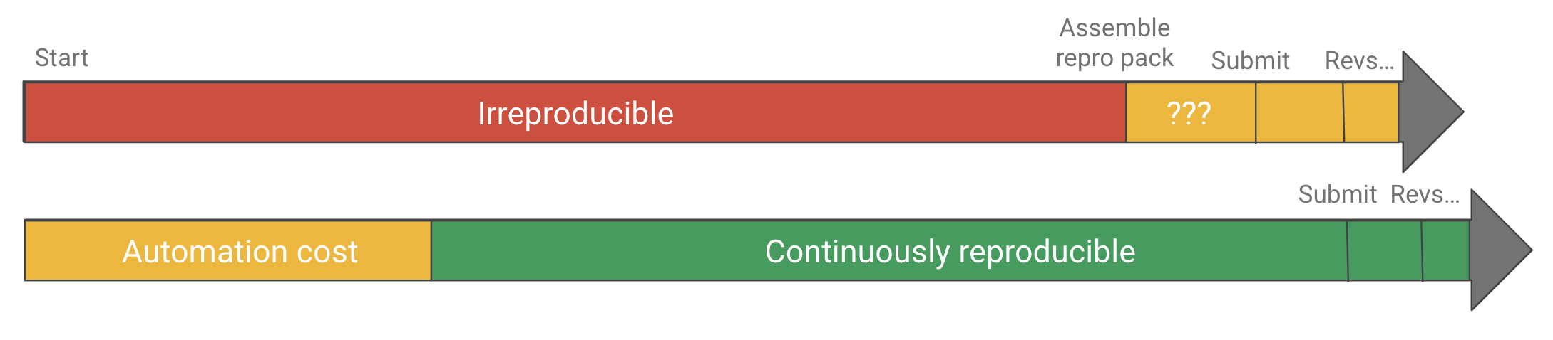
If automation is too costly, it might not be worth it. Driving down the cost
In order to get to a favorable cost/benefit ratio there are a few strategic angles:
- Subsidize the cost:
- Of training
- Of the software engineering and development
- Build tools and infrastructure to bring the cost down
Option 1.1 is the approach of groups like The Carpentries and The Turing Way and it’s a good one. Computational competency may not fit into most curricula, but it can improve the productivity of virtually any knowledge worker, and is therefore worth pursuing.
Option 1.2 is a bit newer, with research software engineer (RSE) becoming a more common job title in academia (my current one, as a matter of fact). The idea is to formalize and pay for the expertise so scientists don’t need to do so much on their own. I like this one as well, and not just because it’s currently how I make a living. Besides teaching and promoting software engineering best practices, RSEs can help scientists turn their newly discovered knowledge into software products to maximize value and impact.
But what about more general tooling and infrastructure to bring down the cost of reproducibility?
There’s a principle in software engineering where once you’ve done something the hard or verbose way a few times, it’s worth building a higher level abstraction for it so it can be used in additional contexts (scaled) more easily. Looking at the current reproducible research stack and best practices it’s clear we’re asking researchers to do things the hard way over and over again, and therefore missing such an abstraction.
The hypothesis is that there must be a way to allow researchers to take advantage of the latest and greatest computational tools without needing to be experts in software engineering. There should be a solution that reduces the accidental complexity and eliminates unimportant decisions and other cognitive overhead while retaining the ability to use state-of-the art libraries and applications—and of course naturally integrates them all into a single-button reproducible workflow.
Simplified tooling and infrastructure for single-button reproducibility
Many of the components to build single-button reproducible workflows exist, mostly from the software development world. We don’t need to replace them with some new monolith. We just need something to tie them all together into a simpler, vertically-integrated, research-focused experience with a gentler learning curve. Basically, assemble all of the components and add some guardrails so researchers don’t have to do it themselves.
Key concepts
Single-button reproducibility can be achieved by following two rules:
- The project is the most important entity, the single source of truth, and should contain all related files. This is sometimes called the “full compendium of artifacts” or the “full knowledge stack” and includes things like code, data, notes, config files, CAD files, figures, tables, and of course the research article. For very large artifacts like datasets, uniquely identifiable pointers can be included in the project to reference remote storage.
- Any derived artifact, e.g., a figure, should not be shared outside the project unless it was produced by its pipeline (the thing that runs with the single button).
Our goal is then to make it easy for researchers to follow these two rules—to create and manage their project and pipeline without becoming de facto software engineers. Now let’s discuss some of the more specific challenges and strategies for overcoming them.
Challenge 1: Version control
Because a project’s inputs, process definitions, and outputs will change over time, and those outputs will be delivered at different point along the project lifecycle, it’s important to keep a history of changes. This history is managed by doing version control, which is also critical for collaboration, allowing people to work concurrently on the same files, i.e., not needing to wait for each other like an assembly line.
Seasoned (and probably elitist) software engineers will say “let them use Git!” However, besides being notoriously complex and difficult to learn, Git is also not ideal for large files or binary files that change often, which will almost certainly be present in a research project. There are solutions out there that make up for this shortcoming, e.g., Large File Storage (LFS), git-annex, and DVC, but all of these require some level of configuration and in some cases additional infrastructure such as S3 buckets or web servers. Our goal is to not require scientists to be software engineers, and so naturally we also don’t want to require them to be cloud computing administrators.
What I propose is something akin to training wheels for Git with support for large files built in. Git provides a solid and performant back end. It just needs a transparent but opinionated wrapper on top to provide an onramp with a simpler interface to get beginners used to saving the full histories of their projects. Once users feel comfortable using it in easy mode, they can start doing more advanced things if desired.
These days, GitHub is the most common place to share Git repositories, and researchers will typically use GitHub to host their code (because GitHub is designed software development), siloing it from the rest of the project materials. What we need is a GitHub for research—a place to store, collaborate on, and share research projects (all files, not just code) throughout their entire lifecycle. Further, the platform’s data model needs to be tailored to the domain. Instead of interacting with repos, forks, and commits, we need an app that deals with figures, datasets, and publications. Hugging Face has done something similar for machine learning.
Lastly, it’s important that this new platform be fully open source (GitHub is not, unfortunately). Centralization of control is antithetical to the principles of open science and presents a significant sustainability risk.
Challenge 2: Tooling fragmentation
It’s important to use the right tool for the job, but in order to achieve single-button reproducibility all tools need to somehow be tied together. Researchers may also need to run different processes in different locations. For example, a simulation may be run on a high performance computing (HPC) cluster, the results post-processed and visualized on a laptop, then written about on a cloud platform like Overleaf. In a single-button reproducible workflow a change to the simulation parameters results in updated figures and tables in the paper without manually moving files around and picking which scripts to run.
We need a way to connect all of these different tools together so researchers don’t need to hop around and manually transfer data between them. We need the project to remain the single source of truth but be able to sync with these more specialized tools. We’ll likely need to integrate, not necessarily replace, things like Google Docs, Sheets, Slides, Microsoft Office, and Google Colab. Importantly, in order to be beginner-friendly, we need a graphical user interface (GUI) that enables data collection, exploration, analysis, and writing all in one place, with an intuitive way to build and run the project’s pipeline and keep track of version history.
Challenge 3: Dependency management
One of the biggest causes of irreproducibility is mutation of (read: installing things in) the user’s global system environment without proper tracking. In other words, they install a variety of apps and libraries to get something working but can’t remember or explain how to do it again. For example, they may run
pip install ...to install a package in their system Python environment and forget about it, or loosely document that in the project’s README. All of their scripts and notebooks may run just fine on their machine but fail on others’.The status quo solution, e.g., for Python projects, is to use a virtual environment. However, even these can be problematic and confusing with typical tools promoting a create-and-mutate kind of workflow. That is, a virtual environment is created, activated, then mutated by installing some packages in it. It’s quite easy to add or update packages without documenting them e.g., in a
requirements.txt. It requires discipline (cognitive overhead) from the user to ensure they properly document the virtual environment. It even requires discipline to ensure it’s activated before running something!# Create a virtual environment python -m venv .venv # Activate it, and remember to activate it every time! source .venv/bin/activate # Now mutate the environment pip install -r requirements.txt # Now what if I mutate further and forget to document? pip install something-elseMore modern environment managers like uv and Pixi automate some of this, making it easy to run a command in a virtual environment and automatically exporting a so-called “lock file” to describe its exact state, not what the user thought it was. However, since these tools are designed for software projects, they typically assume you’ll be working in a single programming language or at least using a single package repository. For research projects, this assumption is often invalid. For example, a user may want to do some statistical calculations in R, some machine learning in Python, then compile a paper with LaTeX, all within the scope of a single project.
Instead of locking users in to a single ecosystem, there should be a project format and manager that allows different environment types, e.g., Python, Docker, R, Julia, or even MATLAB, to be used for different parts of the workflow, and provides a similar interface to create, update, and use each. Users should not be forced to check if environments match their specification, nor should they be expected to document them manually. They should be able to simply define and run.
Challenge 4: Bridging the interactive–batch divide
When writing music, you can spend a long time writing it all out on paper, imagining what it will sound like, then have someone play it at the end, or you can sit at the instrument and keep playing until it sounds right. The latter—an interactive workflow—is more intuitive, with faster feedback and shorter iteration cycle time. Interactive workflows are great ways to discover ideas, but once a valuable creation has been discovered, it needs to be written down or recorded so it can be reproduced in a batch process. The same is true for creating a figure or transforming some data.
This problem is similar to dependency management. When working interactively, it’s possible to arrive at an output you like while losing track of how you got there. And so here’s the challenge: How do we allow researchers to experiment with different ideas for data processing or visualization in an interactive way but also get them to “record” what they did so it can be edited and replayed later?
Following our second rule of single-button reproducibility, we need to get researchers to produce derived artifacts with a project’s pipeline before sharing. It therefore needs to be easier to automate the creation of a figure than it is to simply copy and paste it into some slides and email them out. What we need is a pipeline that is easy to create, update, and understand. Users need to be able to run something like a Jupyter notebook interactively to explore how it might work best, add it to the pipeline, and run the project to see if it properly produces the thing they’d like to share.
The pipeline also needs to be able to run quickly so users don’t need to think about which stages need to be run—that would be a multi-button workflow. In other words, it will need to cache outputs and only rerun stages when the cache becomes invalidated.
Lastly, the collaboration platform on which they’re working (the “GitHub for science”) should make it easy to share artifacts from the pipeline so it’s less tempting to export one generated interactively.
If we build it…
Automation presents a huge potential for increasing the pace (and reducing the stress) of scientific discovery, but the cost of single-button reproducibility—the standard we should strive for—is still too high for most researchers. Many simply don’t have the time or desire to become de facto software engineers, and that’s okay. We need to include them too. In addition to providing training and support, we need to meet them in the middle with a less software development-oriented, more research-oriented and user-friendly set of tools and infrastructure.
Calkit is a start down this path, but there is still much to do. If you’re a researcher excited by the prospect of fully automated workflows and the peace of mind they bring, consider joining the project as a design partner. You’ll get free “reproducibility support” and any ideas we discover will be fed back into the software so others can benefit. Similarly, if you’re a software developer and this vision resonates with you, consider getting involved.
-
March 17, 2025
Continuous Reproducibility: How DevOps principles could improve the speed and quality of scientific discovery
In the 21st century, the Agile and DevOps movements revolutionized software development, reducing waste, improving quality, enhancing innovation, and ultimately increasing the speed at which software products were brought into the world. At the same time, the pace of scientific innovation appears to have slowed [1], with many findings failing to replicate (validated in an end-to-end sense by reacquiring and reanalyzing raw data) or even reproduce (obtaining the same results by rerunning the same computational processes on the same input data). Science already borrows much from the software world in terms of tooling and best practices, which makes sense since nearly every scientific study involves computation, but there are still more yet to cross over.
Here I will focus on one set of practices in particular: those of Continuous Integration and Continuous Delivery (CI/CD). There has been some discussion about adapting these under the name Continuous Analysis [2], though since the concept extends beyond analysis and into generating other artifacts like figures and publications, here I will use the term Continuous Reproducibility (CR).
CI means that valuable changes to code are incorporated into a single source of truth, or “main branch,” as quickly as possible, resulting in a continuous flow of small changes rather than in larger, less frequent batches. CD means that these changes are accessible to the users as soon as possible, e.g., daily instead of quarterly or annual “big bang” releases.
CI/CD best practices ensure that software remains working and available while evolving, allowing the developers to feel safe and confident about their modifications. Similarly, CR would ensure the research project remains reproducible—its output artifacts like datasets, figures, slideshows, and publications, remain consistent with input data and process definitions—hypothetically allowing researchers to make changes more quickly and in smaller batches without fear of breaking anything.
But CI and CD did not crop up in isolation. They arose as part of a larger wave of changes in software development philosophy.
In its less mature era, software was built using the traditional waterfall project management methodology. This approach broke projects down into distinct phases or “stage gates,” e.g., market research, requirements gathering, design, implementation, testing, deployment, which were intended to be done in a linear sequence, each taking weeks or months to finish. The industry eventually realized that this only works well for projects with low uncertainty, i.e., those where the true requirements can easily be defined up front and no new knowledge is uncovered between phases. These situations are of course rare in both product development and science.
These days, in the software product world, all of the phases are happening continuously and in parallel. The best teams are deploying new code many times per day, because generally, the more iterations, the more successful the product.
But it’s only possible to do many iterations if cycle times can be shortened. In the old waterfall framework, full cycle times were on the order of months or even years. Large batches of work were transferred between different teams in the form of documentation—a heavy and sometimes ineffective communication mechanism. Further, the processes to test and release software were manual, which meant they could be tedious, expensive, and/or error prone, providing an incentive to do them less often.
One strategy that helped reduce iteration cycle time was to reduce communication overhead by combining development and operations teams (hence “DevOps”). This allowed individuals to simply talk to each other instead of handing off formal documentation. Another crucial tactic was the automation of test and release processes with CI/CD pipelines. Combined, these made it practical to incorporate fewer changes in each iteration, which helped to avoid mistakes and deliver value to users more quickly—a critical priority in a competitive marketplace.
I’ve heard DevOps described as “turning collaborators into contributors.” To achieve this, it’s important to minimize the amount of effort required to get set up to start working on a project. Since automated CI/CD pipelines typically run on fresh or mostly stateless virtual machines, setting up a development/test environment needs to be automated, e.g., with the help of containers and/or package managers. These pipelines then serve as continuously tested documentation, which can be much more reliable than a list of steps written in a README.
So how does this relate to research projects, and are there potential efficiency gains to be had if similar practices were to be adopted?
In research projects we certainly might find ourselves thinking in a waterfall mindset, with a natural inclination to work in distinct, siloed phases, e.g., planning, data collection, data analysis, figure generation, writing, peer review. But is a scientific study really best modeled as a waterfall process? Do we never, for example, need to return to data analysis after starting the writing or peer review?
Instead, we could think of a research project as one continuous iterative process. Writing can be done the entire time in small chunks. For example, we can start writing the introduction to our first paper and thesis from day one, as we do our literature review. The methods section of a paper can be written as part of planning an experiment, and updated with important details while carrying it out. Data analysis and visualization code can be written and tested before data is collected, then run during data collection as a quality check. Instead of thinking of the project as a set of decoupled sub-projects, each a big step done one after the other, we could think of the whole thing as one unit that evolves in small steps.
Similar to how software teams work, where an automated CD pipeline will build all artifacts, such as compiled binaries or minified web application code, and make them available to the users, we can build and deliver all of our research project artifacts each iteration with an automated pipeline, keeping them continuously reproducible. (Note that in this case “deliver” could mean to our internal team if we haven’t yet submitted to a journal.)
In any case, the correlation between more iterations and better outcomes appears to be mostly universal for all kinds of endeavors, so at the very least, we should look for behaviors that are hurting research project iteration cycle time. Here are a few DevOps-related ones I can think of:
Problem or task Slower, more error-prone solution ❌ Better solution ✅ Ensuring everyone on the team has access to the latest version of a file as soon as it is updated, and making them aware of the difference from the last version. Send an email to the whole team with the file and change summary attached every time a file changes. Use a single shared version-controlled repository for all files and treat this as the one source of truth. Updating all necessary figures and publications after changing data processing algorithms. Run downstream processes manually as needed, determining the sequence on a case-by-case basis. Use a pipeline system that tracks inputs and outputs and uses caching to skip unnecessary expensive steps, and can run them all with a single command. Ensuring the figures in a manuscript draft are up-to-date after changing a plotting script. Manually copy/import the figure files from an analytics app into a writing app. Edit the plotting scripts and manuscript files in the same app (e.g., VS Code) and keep them in the same repository. Update both with a single command. Showing the latest status of the project to all collaborators. Manually create a new slideshow for each update. Update a single working copy of the figures, manuscripts, and slides as the project progresses so anyone can view asynchronously. Ensuring all collaborators can contribute to all aspects of the project. Make certain tasks only able to be done by certain individuals on the team, and email each other feedback for updating these. Use a tool that automatically manages computational environments so it’s easy for anyone to get set up and run the pipeline. Or better, run the pipeline automatically with a CI/CD service like GitHub Actions. What do you think? Are you encountering these sorts of context switching and communication overhead losses in your own projects? Is it worth the effort to make a project continuously reproducible? I think it is, though I’m biased, since I’ve been working on tools to make it easier (Calkit; cf. this example CI/CD workflow).
One argument you might have against against adopting CR in your project is that you do very few “outer loop” iterations. That is, you are able to effectively work in phases so, e.g., siloing the writing away from the data visualization is not slowing you down. I would argue, however, that analyzing and visualizing data concurrently while it’s being collected is a great way to catch errors, and the earlier an error is caught, the cheaper it is to fix. If the paper is set up and ready to write during data collection, important details can make their way in directly, removing a potential source of error from transcribing lab notebooks.
---
title: Outer loop(s)
---
flowchart LR
    A[collect data] --> B[analyze data]
    B --> C[visualize data]
    C --> D[write paper]
    D --> A
    C --> A
    D --> C
    D --> B
    C --> B
    B --> D
    B --> A
--- title: Inner loop --- flowchart LR A[write] --> B[run] B --> C[review] C --> AUsing Calkit or a similar workflow like that of showyourwork, one can work on both outer and inner loop iterations in a single interface, e.g., VS Code, reducing context switching costs.
On the other hand, maybe the important cycle time(s) are not for iterations within a given study, but at a higher level—iterations between studies themselves. However, one could argue that delivering a fully reproducible project along with a paper provides a working template for the next study, effectively reducing that “outer outer loop” cycle time.
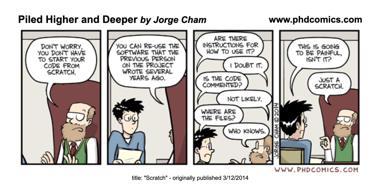
If CR practices make it easy to get set up and run a project, and again, the thing actually works, perhaps the next study can be done more quickly. At the very least, the new project owner will not need to reinvent the wheel in terms of project structure and tooling. Even if it’s just one day per study saved, imagine how that compounds over space and time. I’m sure you’ve either encountered or heard stories of grad students being handed code from their departed predecessors with no instructions on how to run it, no version history, no test suite, etc. Apparently that’s common enough to make a PhD Comic about it:
If you’re convinced of the value of Continuous Reproducibility—or just curious about it—and want help implementing CI/CD/CR practices in your lab, shoot me an email, and I’d be happy to help.
References and recommended resources
- Nicholas Bloom, Charles I Jones, John Van Reenen, and Michael Web (2020). Are Ideas Getting Harder to Find? American Economic Review. 10.1257/aer.20180338
- Brett K Beaulieu-Jones and Casey S Greene (2017). Reproducibility of computational workflows is automated using continuous analysis. Nat Biotechnol. 10.1038/nbt.3780
- Toward a Culture of Computational Reproducibility. https://youtube.com/watch?v=XjW3t-qXAiE
- There is a better way to automate and manage your (fluid) simulations. https://www.youtube.com/watch?v=NGQlSScH97s