Reproducible OpenFOAM simulations with Calkit

October 23, 2024 | 12 Minute Read

Have you ever been here before? You’ve done a bunch of work to get a simulation to run, created some figures, and submitted a paper to a journal. A month or two later you get the reviews back and you’re asked by the dreaded Reviewer 2 to make some minor modifications to a figure. There’s one small problem, however: You don’t remember how that figure was created, or you’ve upgraded your laptop and now the script won’t run. Maybe you were able to clone the correct Git repo with the code, but you don’t remember where the data is supposed to be stored. In other words, your project is not reproducible.

Here we are going to show how to make a research project reproducible with Calkit, a tool I’ve been working on that ties together and simplifies a few lower-level tools to help with reproducibility:

• Git
• GitHub
• DVC (Data Version Control)
• Docker
• Cloud storage

We’re going to use OpenFOAM and Python to generate our outputs since these both can be pretty tricky to get setup correctly, never mind setup correctly twice!

Getting setup

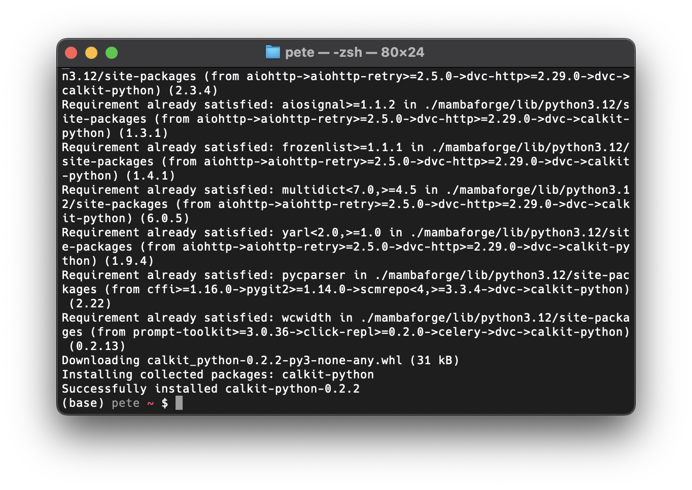
You will need to have Git installed, and you’ll need to have a GitHub account. You’ll also need to have Python (Mambaforge recommended) and Docker installed. After that, install the Calkit Python package with:

pip install calkit-python

Creating and cloning the project repo

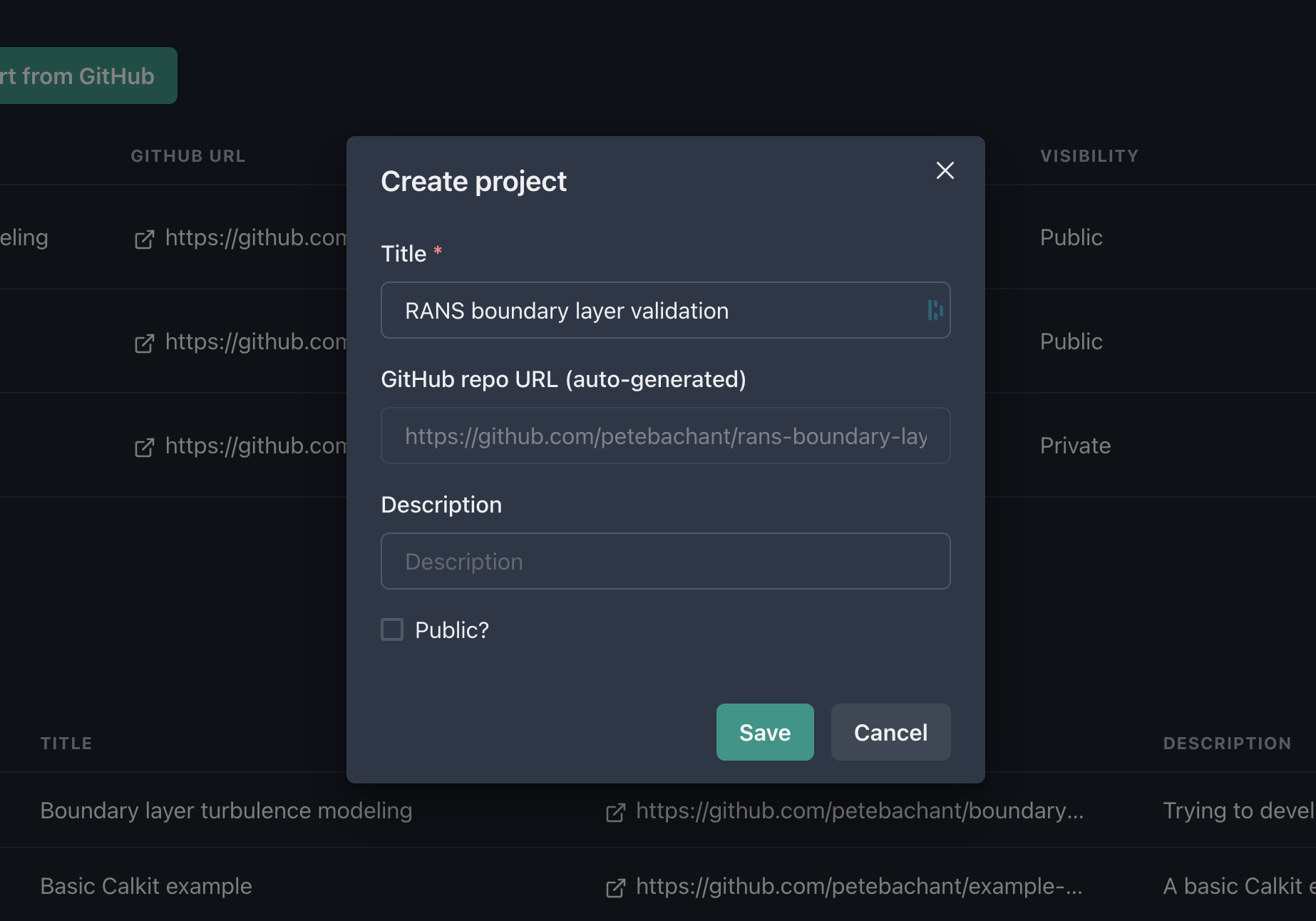
Head over to calkit.io and log in with your GitHub account. Click the button to create a new project. Let’s title ours “RANS boundary layer validation”, since for our example, we’re going to create a project that attempts to answer the question:

What RANS model works best for a simple boundary layer?

We’ll keep this private for now (though in general it’s good to work openly.) Note that creating a project on Calkit also creates the project Git repo on GitHub.

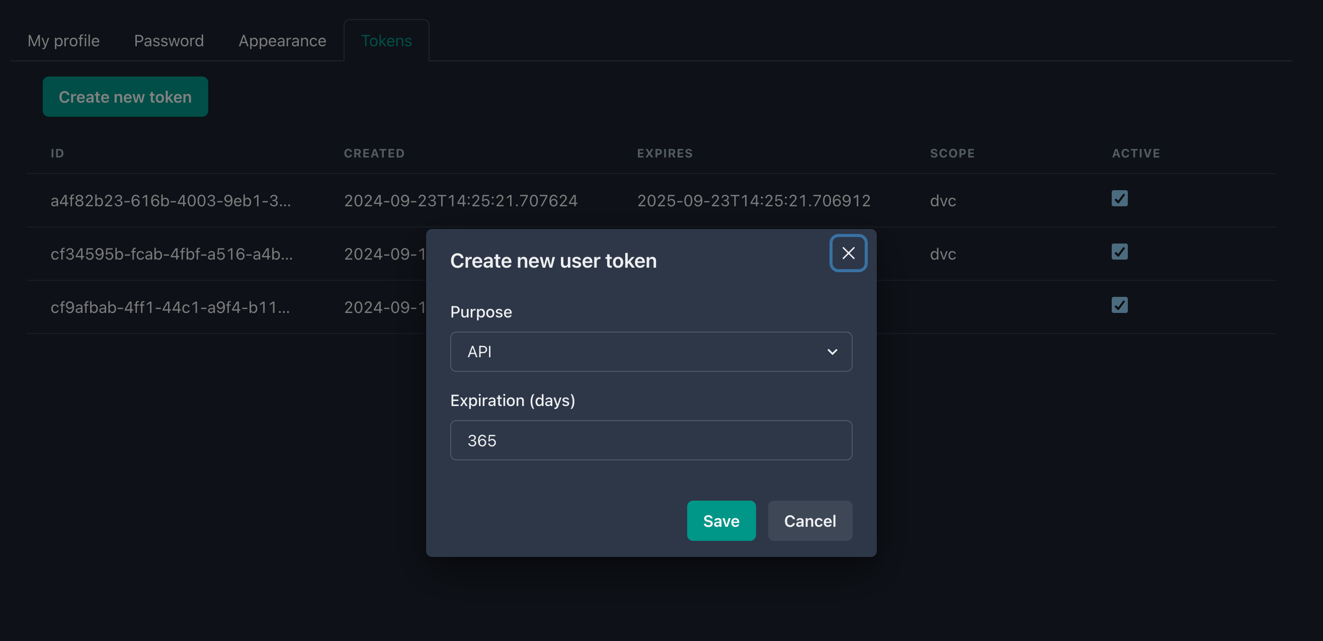
We’re going to need a token to interact with the Calkit API, so head over to your user settings, generate one for use with the API, and copy it to your clipboard.

Then we can set that token in our Calkit configuration with:

calkit config set token YOUR_TOKEN_HERE

Next, clone the repo to your local machine with (filling in your username):

calkit clone https://github.com/YOUR_USERNAME/rans-boundary-layer-validation.git

Note you can modify the URL above to use SSH if that’s how you interact with GitHub.

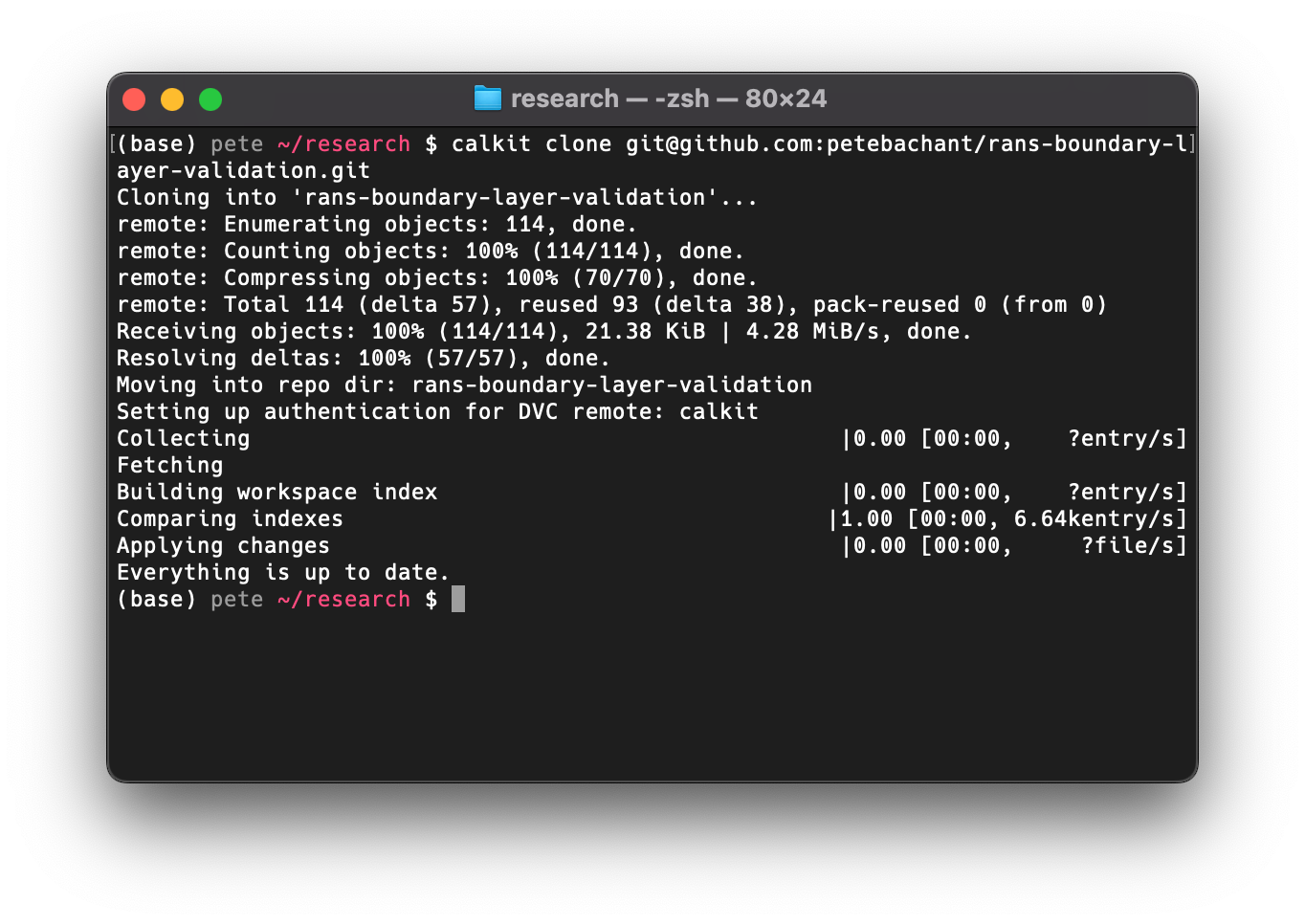
calkit clone is a simple wrapper around git clone that sets up the necessary configuration to use the Calkit Cloud as a DVC remote, the place where we’re going to push our data, while our code goes to GitHub.

Getting some validation data

We want to validate these RANS models, so we’ll need some data for comparison. It just so happens that there is already a boundary layer direct numerical simulation (DNS) dataset on Calkit downloaded from the Johns Hopkins Turbulence Databases (JHTDB), so we can simply import that with (after cding into the project directory):

calkit import dataset \
    petebachant/boundary-layer-turbulence-modeling/data/jhtdb-transitional-bl/time-ave-profiles.h5 \
    data/jhtdb-profiles.h5

If we run calkit status we can see that there is one commit that has been made but not pushed to origin/main (on GitHub), so we can make sure everything is backed up there with calkit push.

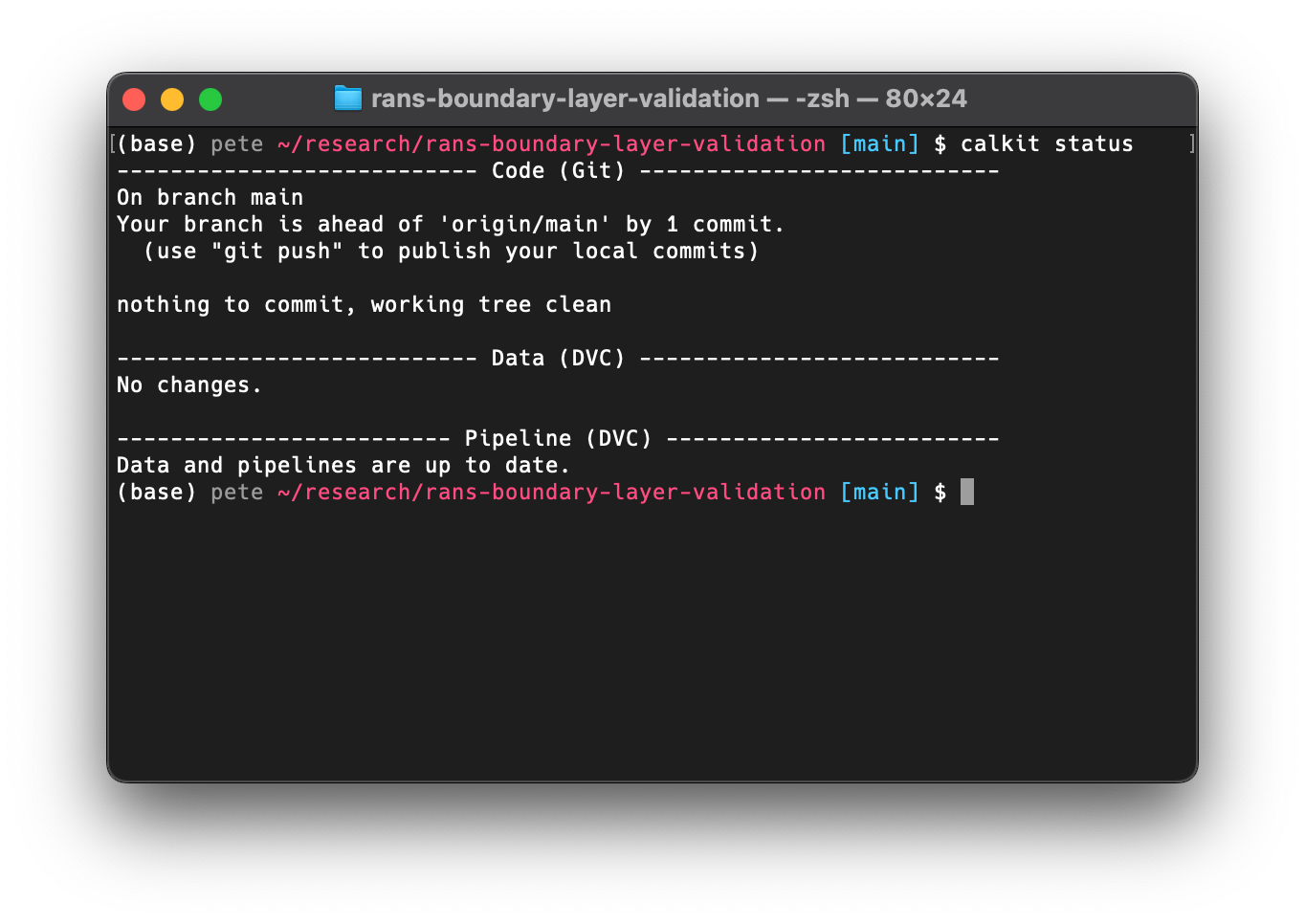
calkit status and calkit push behave very similarly to git status and git push. In fact, those commands are run alongside some additional DVC commands, the importance of which we will see shortly.

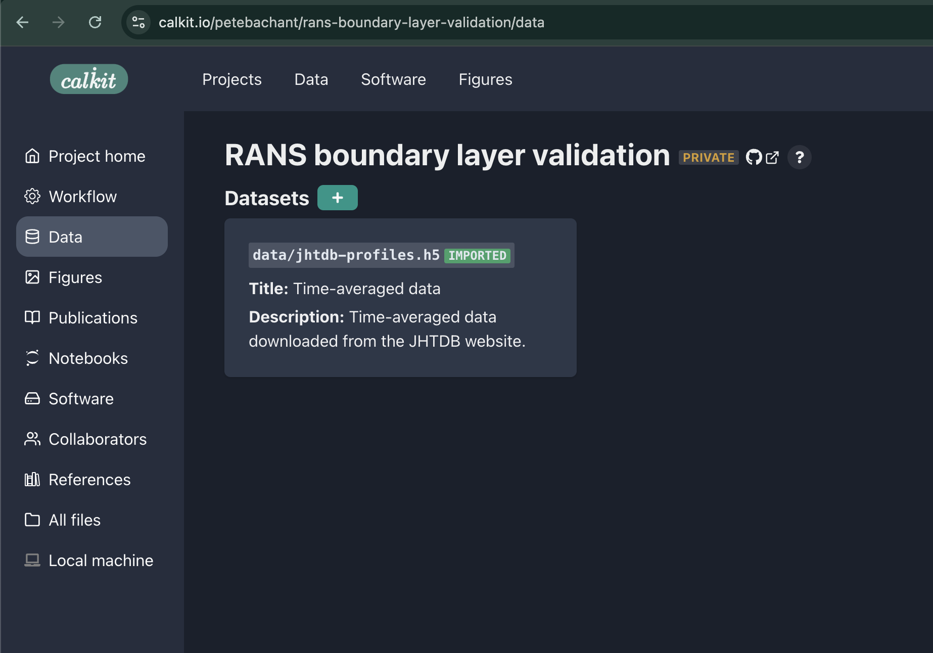
We can now see our imported dataset as part of the project datasets on the Calkit website. We can also see the file is present, but ignored by Git, since it’s managed by DVC. Because the dataset was imported, it does not take up any of this project’s storage space, but will be present when the repo is cloned.

Creating a reproducible OpenFOAM environment with Docker

If you’ve never worked with Docker, it can sound a bit daunting, but Calkit has some tooling to make it a bit easier. Basically, Docker is going to let us create isolated reproducible environments in which to run commands and will keep track of which environments belong to this project in the calkit.yaml file.

Let’s create an OpenFOAM-based Docker environment and build stage with:

calkit new docker-env \
    --name foam \
    --image openfoam-2406-foampy \
    --stage build-docker \
    --from microfluidica/openfoam:2406 \
    --add-layer mambaforge \
    --add-layer foampy \
    --description "OpenFOAM v2406 with foamPy."

This command will create the necessary Dockerfile, the environment in our project metadata, and will add a stage to our DVC pipeline to build the image before running any other commands.

If we run calkit status again, we see that there’s another commit to be pushed to GitHub, and our pipeline is showing some changed dependencies and outputs.

This is a signal that it is out-of-date, and should be executed with calkit run. When we do that we see some output from Docker as an image is built, and calkit status then shows we have a new dvc.lock file staged and an untracked Dockerfile-lock.json file.

We’ll need to add that Dockerfile-lock.json file to our repo and then commit and push to the cloud so it is backed up and accessible to our collaborators. We can do this with the calkit save command:

calkit save dvc.lock Dockerfile-lock.json -m "Run pipeline to build Docker image"

which does the add, commit, push steps all in one, deciding which files to store in DVC versus Git, and pushing to the respective locations to save time and cognitive overhead. However, if desired, you can of course run those individually for full control.

Finally, let’s check that we can run something in the environment, e.g., print the help output of blockMesh:

calkit runenv -- blockMesh -help

Now we’re good to go. We didn’t need to install OpenFOAM, and neither will our collaborators. We’re now ready to start setting up the cases.

Adding the simulation runs to the pipeline

We can run things interactively and make sure things work, but it’s not a good idea to rely on interactive or ad hoc processes to produce a permanent artifact. Any time you get to a point where you do want to save something permanent, the pipeline should be updated to produce that artifact, so let’s add some simulation runs to ours.

We want to run the simulation to validate a few different turbulence models:

• Laminar (no turbulence model)
• $k$–$\epsilon$
• $k$–$\omega$

I’ve setup this project to use foamPy to create and run variants of a case with a “templatized” turbulenceProperties file via a script run.py, which we’re going to run in our Docker environment.

To simulate the same case for multiple turbulence models, we’re going to create a “foreach” DVC stage to run our script over a sequence of values. When setup properly, DVC will be smart enough to cache the results and not rerun simulations when they don’t need to be rerun. We can create this stage with:

calkit new foreach-stage \
    --cmd "calkit runenv python run.py --turbulence-model {var} -f" \
    --name run-sim \
    --dep system \
    --dep constant/transportProperties \
    --dep run.py \
    --dep Dockerfile-lock.json \
    --out "cases/{var}/postProcessing" \
    "laminar" "k-epsilon" "k-omega"

Another call to calkit status shows our pipeline needs to be run, which makes sense, so let’s give it another calkit run. You’ll note at the very start our Docker image build stage is not rerun thanks to DVC tracking and caching the inputs and outputs.

The output of calkit status now shows something we haven’t seen yet: we have some new data produced as part of those simulation runs. We can do another calkit save to ensure everything is committed and pushed:

calkit save -am "Run simulations"

In this case, the outputs of the simulations were pushed up to the DVC remote in the Calkit Cloud.

We are defining an output for each simulation as the postProcessing folder, which we will cache and push to the cloud for backup, so others (including our future self), can pull down the results and work with them without needing to rerun the simulations. We are also defining dependencies for the simulations. What this means is that if anything in the system folder, the run.py script, constant/transportProperties, or our Dockerfile changes, DVC will know it needs to rerun the simulations. Conversely, if those haven’t changed and we already have results cached, there’s no need to rerun. This is nice because to produce our outputs we basically only need to remember one command and keep running it, and that’s simply calkit run, which is a wrapper around dvc repro that parses some additional metadata to define certain special objects, e.g., datasets or figures.

Creating a figure to visualize our results

We want to compare the OpenFOAM results to the DNS data, for which we can plot the mean streamwise velocity profiles, for example. We can create a new figure with its own pipeline stage with:

calkit new figure \
    figures/mean-velocity-profiles.png \
    --title "Mean velocity profiles" \
    --description "Mean velocity profiles from DNS and RANS models." \
    --stage plot-mean-velocity-profiles \
    --cmd "calkit runenv python scripts/plot-mean-velocity-profiles.py" \
    --dep scripts/plot-mean-velocity-profiles.py \
    --dep data/jhtdb-profiles.h5 \
    --deps-from-stage-outs run-sim

The last line there is going to automatically create dependencies based on the outputs of our run-sim stage, saving us the trouble of typing out all of those directories manually.

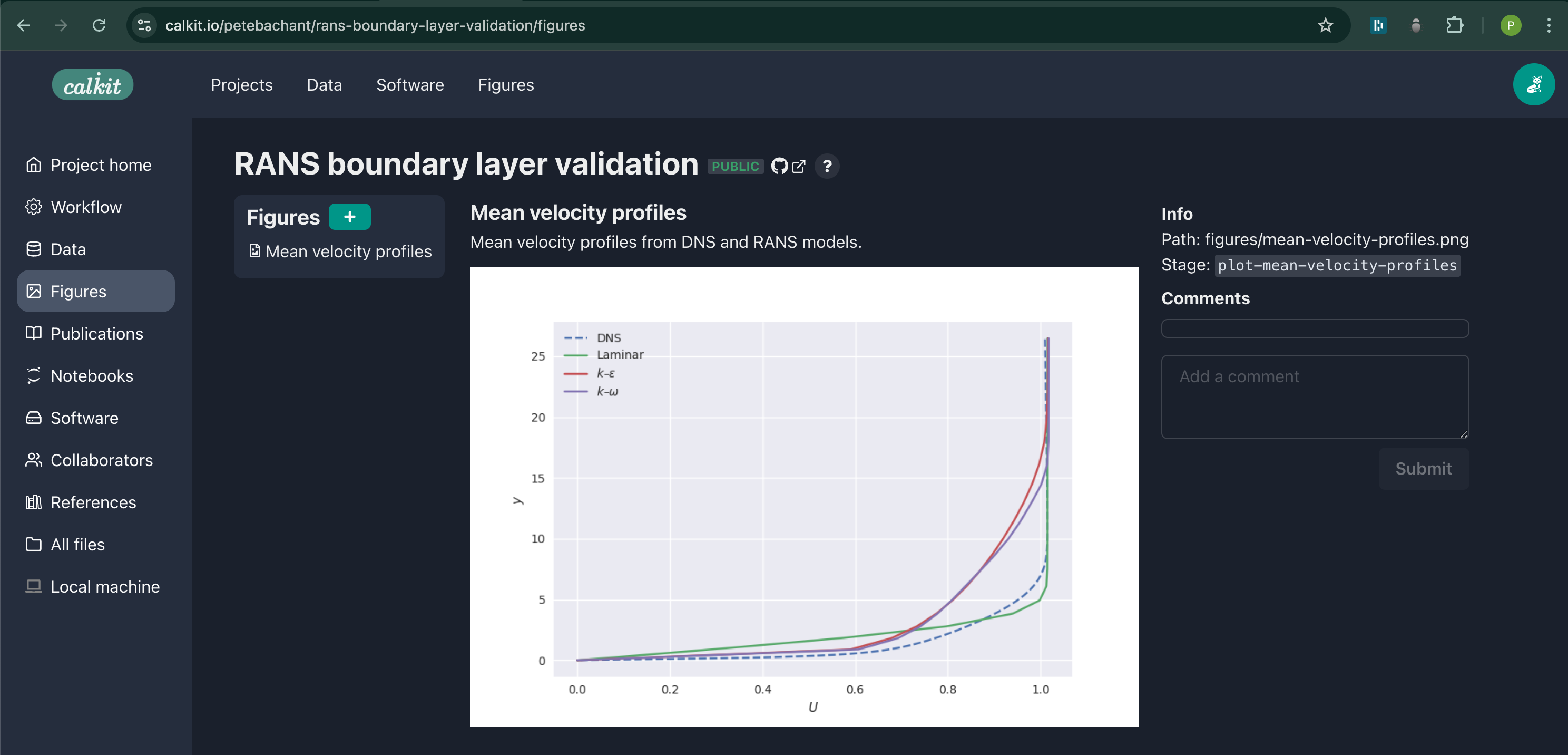
Another call to calkit status shows we need to run the pipeline again, and another call to calkit run then calkit save -m "Run pipeline to create figure" will create this figure and push it to the repo. This figure is now viewable as its own object up on the website:

Solving the problem

Now let’s show the value of making our project reproducible, addressing the problem we laid out in the introduction, assuming Reviewer 2’s request was something like:

The legend labels should be updated to use mathematical symbols.

We’re going to pretend we were forced to start from scratch, so let’s delete the local copy of our project repo and clone it again using same calkit clone command we ran above.

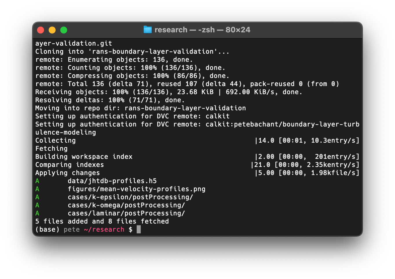
After moving into the freshly cloned repo, you’ll notice our imported dataset, the cases/*/postProcessing directories, and our figure PNG file were all downloaded, which would not have happened with a simple git clone, since those files are kept out of Git.

Running calkit status and calkit run again shows that what we’ve cloned is fully up-to-date.

Next we edit our plotting script to make the relevant changes. Then we execute calkit run. Again, notice how the simulations were not rerun thanks to the DVC cache.

If we run calkit status we see there are some differences, so we run calkit save -am "Change x-axis label for reviewer 2" to get those saved and backed up. If we go visit the project on the Calkit website, we see our figure is up-to-date and has the requested changes in the legend. Reviewer 2 will be so happy 😀

Conclusions and next steps

We created a project that runs OpenFOAM simulations reproducibly, produces a figure comparing against an imported dataset, and ensures these are kept in version control and backed up to the cloud. This is of course a simplified example for demonstration, but you could imagine expanding the pipeline to include more operations, such as:

• Running a mesh independence study.
• Building a LaTeX document as a report or paper.

Since DVC pipelines can run any arbitrary command, you’re not locked into a specific language or framework. You could run shell scripts, MATLAB programs, etc., all in a single pipeline.

You can view this project up on Calkit and GitHub if you’d like to get started doing something similar. Also, please comment below if you’re using a different tool or framework to make your own work reproducible.