Physical and numerical modeling of cross-flow turbines

by Pete Bachant

Advisor: Martin Wosnik

What is a cross-flow turbine?

• Axis perpendicular to flow
• Some success in onshore wind
• Surpassed by HAWTs (AFTs) →
  • Exaggerated power ratings
  • Fatigue issues

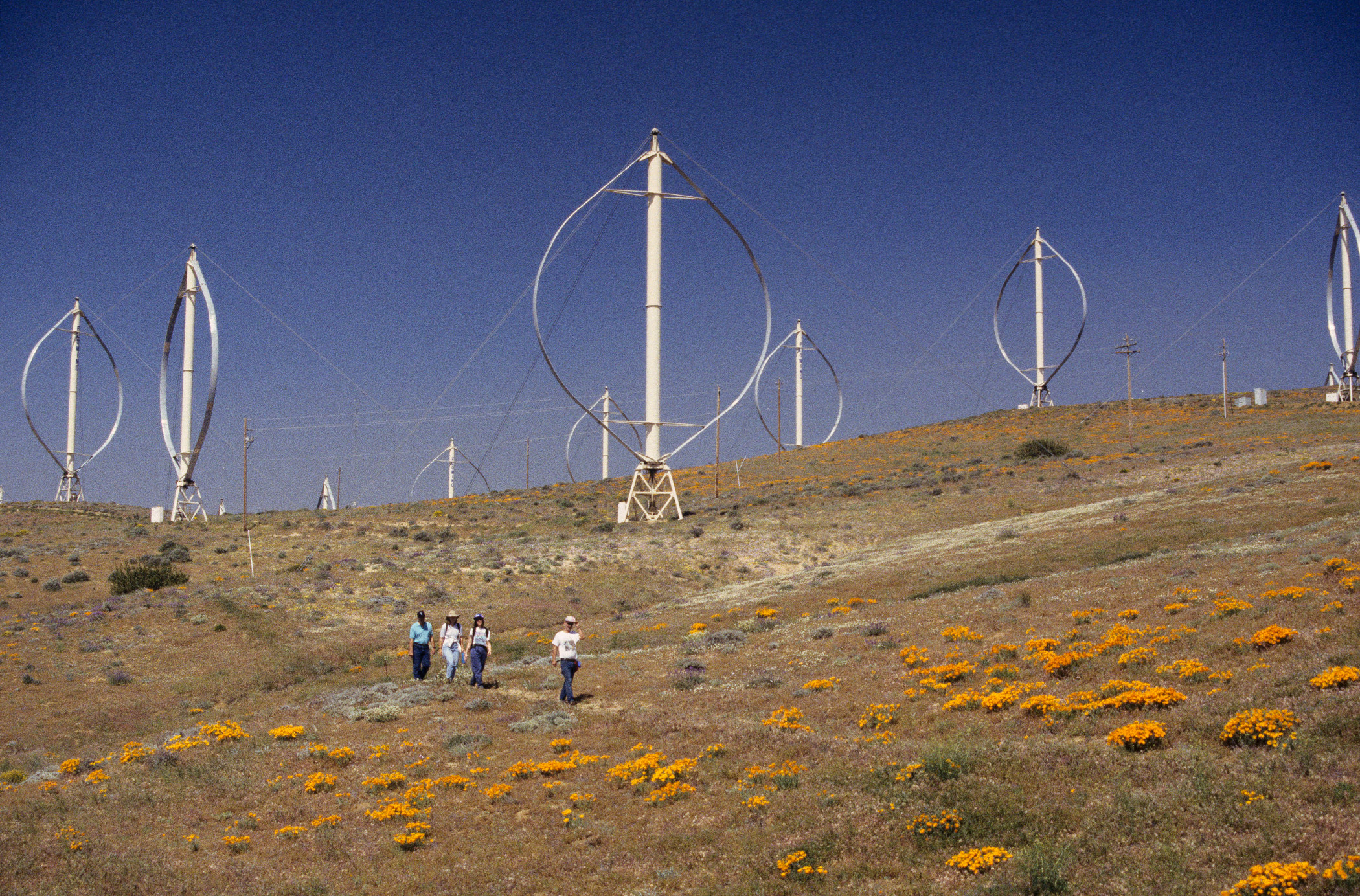
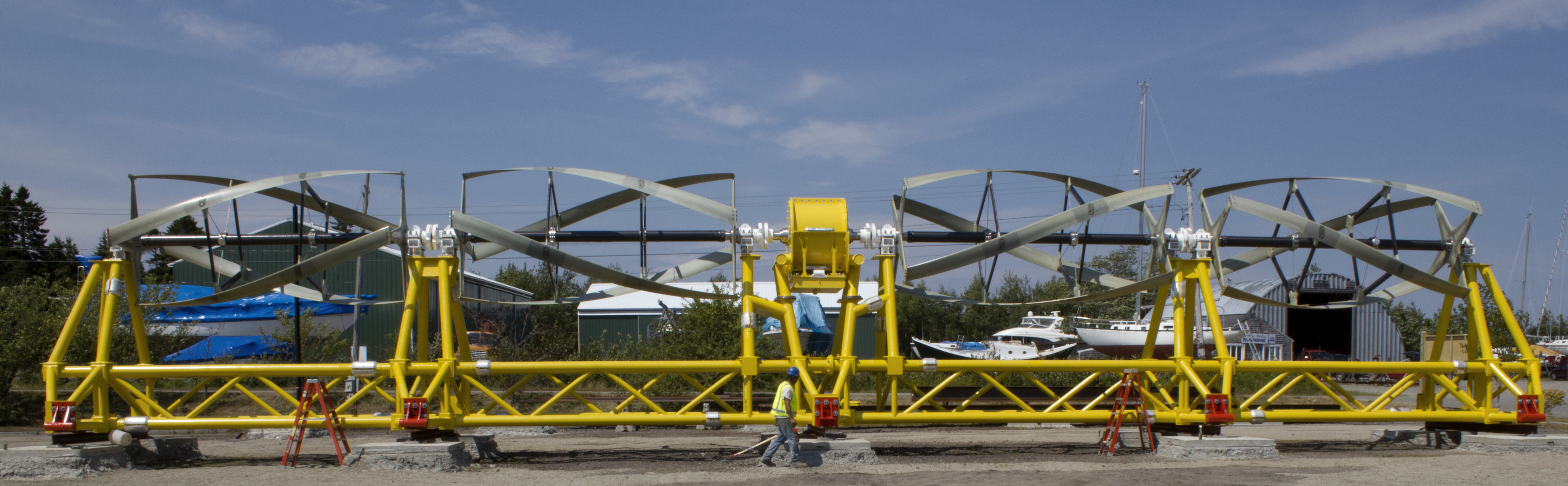
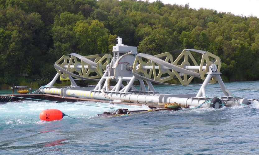
Left: Photo by Paul Gipe. All rights reserved. Upper right: Courtesy of Vestas Wind Systems A/S. Lower right: From Murray and Barone (2011).

Marine hydrokinetics: ORPC

TidGen, Cobscook Bay, ME:

RivGen, Igiugig, AK:

From orpc.co.

• Higher solidity $Nc/(\pi D)$ or $c/R$ than Darrieus VAWTs due to order of magnitude higher torque.
• Imagine how many axial-flow rotors it would take to fit in there

Wind turbine arrays: Caltech FLOWE

Closely spaced VAWTs may achieve higher power output per unit land area compared to HAWTs. Note the rotors shown here are also high solidity.

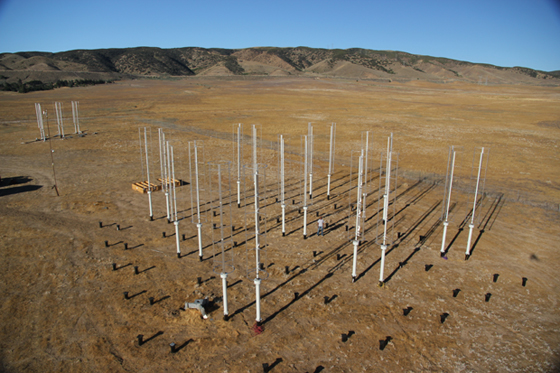
From flowe.caltech.edu.

Blade element theory

Assume kinematics and dynamics act on blade section at one point.

import warnings
warnings.filterwarnings("ignore")
os.chdir(os.path.join(os.path.expanduser("~"), "Google Drive", "Research", "CFT-vectors"))
import cft_vectors
fig, ax = plt.subplots(figsize=(15, 15))
fontsize = plt.rcParams["font.size"]
with plt.rc_context({"font.size": 1.5*fontsize}):
    cft_vectors.plot_diagram(fig, ax, theta_deg=52, axis="off", label=True)
os.chdir(talk_dir)

Blade element theory

In an idealized case, CFT is unsteady, often $\alpha_\max \gt \alpha_{\mathrm{ss}}$. Not so for AFT.

Unsteadiness is more dramatic for higher c/R.

Quantifying unsteadiness

Reduced frequency:

$$ k = \frac{\omega c}{2 U_\infty} = \frac{\lambda c}{2R} $$$$ \lambda = \frac{\omega R}{U_\infty} $$

Unsteady effects significant for $k > 0.05$, dominant for $k \ge 0.2$ [1].

Rotor	$ c/R $	$\lambda$	$k$
Sandia 34 m Darrieus	0.05	6	0.16
Hypothetical MHK	0.25	2	0.25

MHK rotor blades see approximately one order of magnitude higher torque vs. wind.

[1] Leishman (2006) "Principles of Helicopter Aerodynamics", Cambridge.

Research objectives

1. Produce model validation datasets for higher solidity CFTs
2. Investigate near-wake, especially recovery
   • Relevant to array design
3. Evaluate Navier–Stokes based models (blade-resolved and parameterized) for predicting performance and wake characteristics
   • Lower fidelity models fail for higher $c/R$
   • Computing power has advanced tremendously since the Darrieus VAWT R&D

Turbine test bed

Automated turbine testing in the UNH tow tank

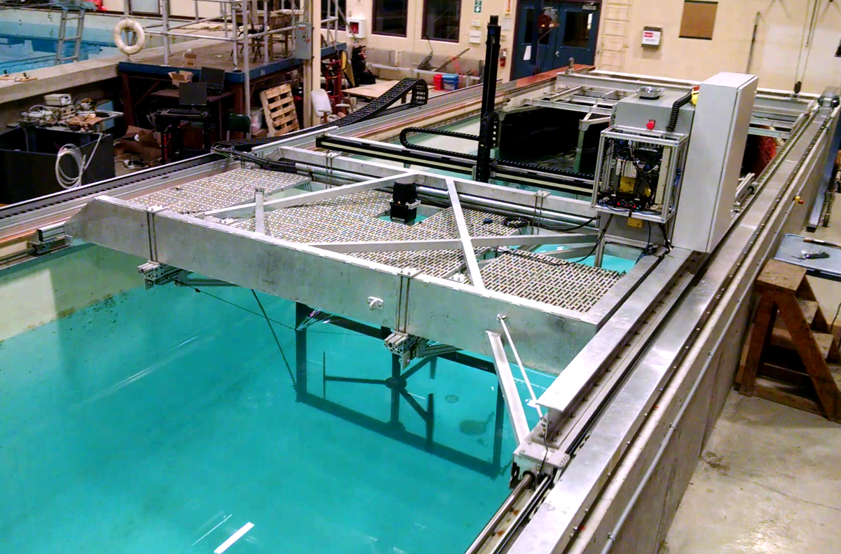
Test bed instrumentation

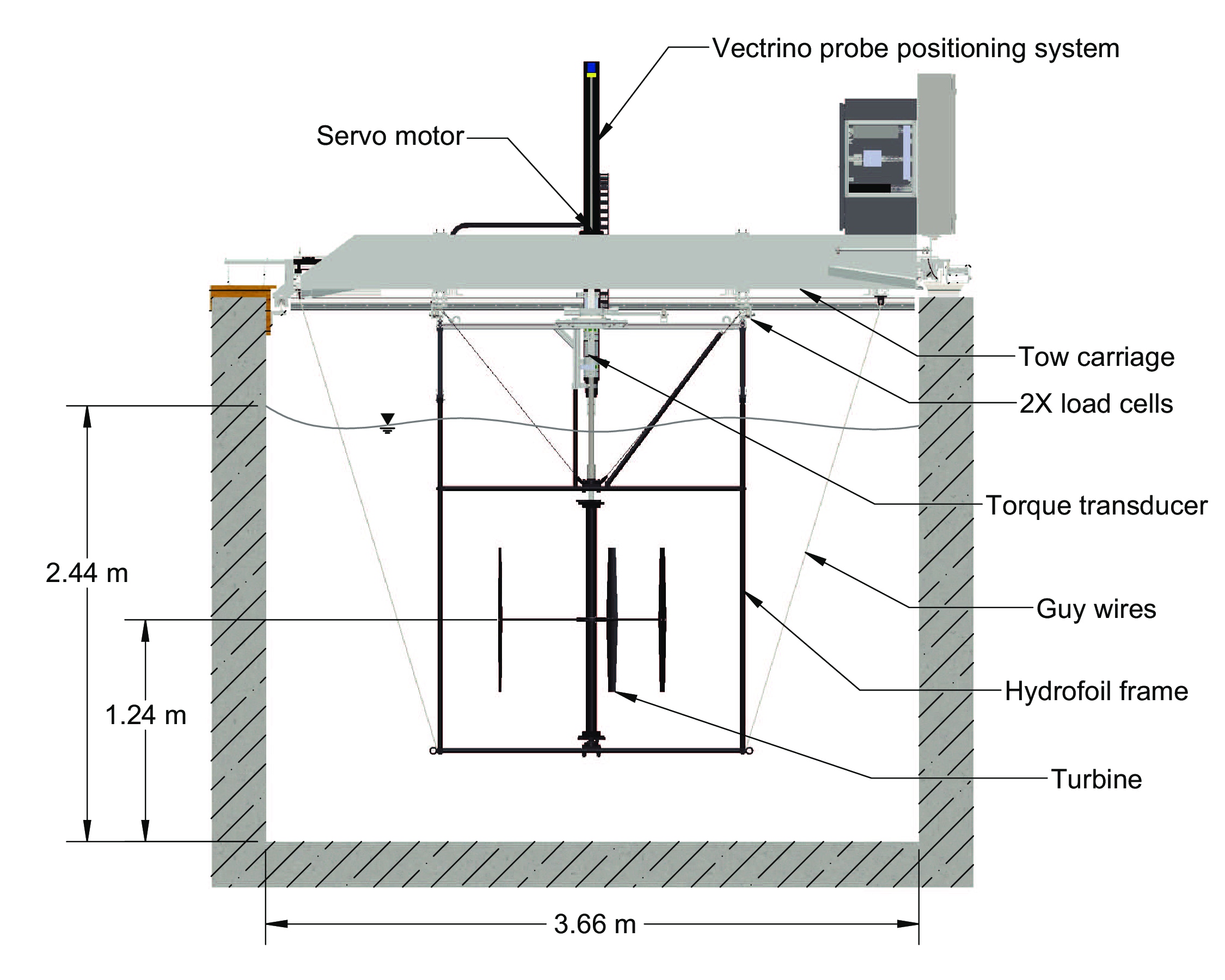
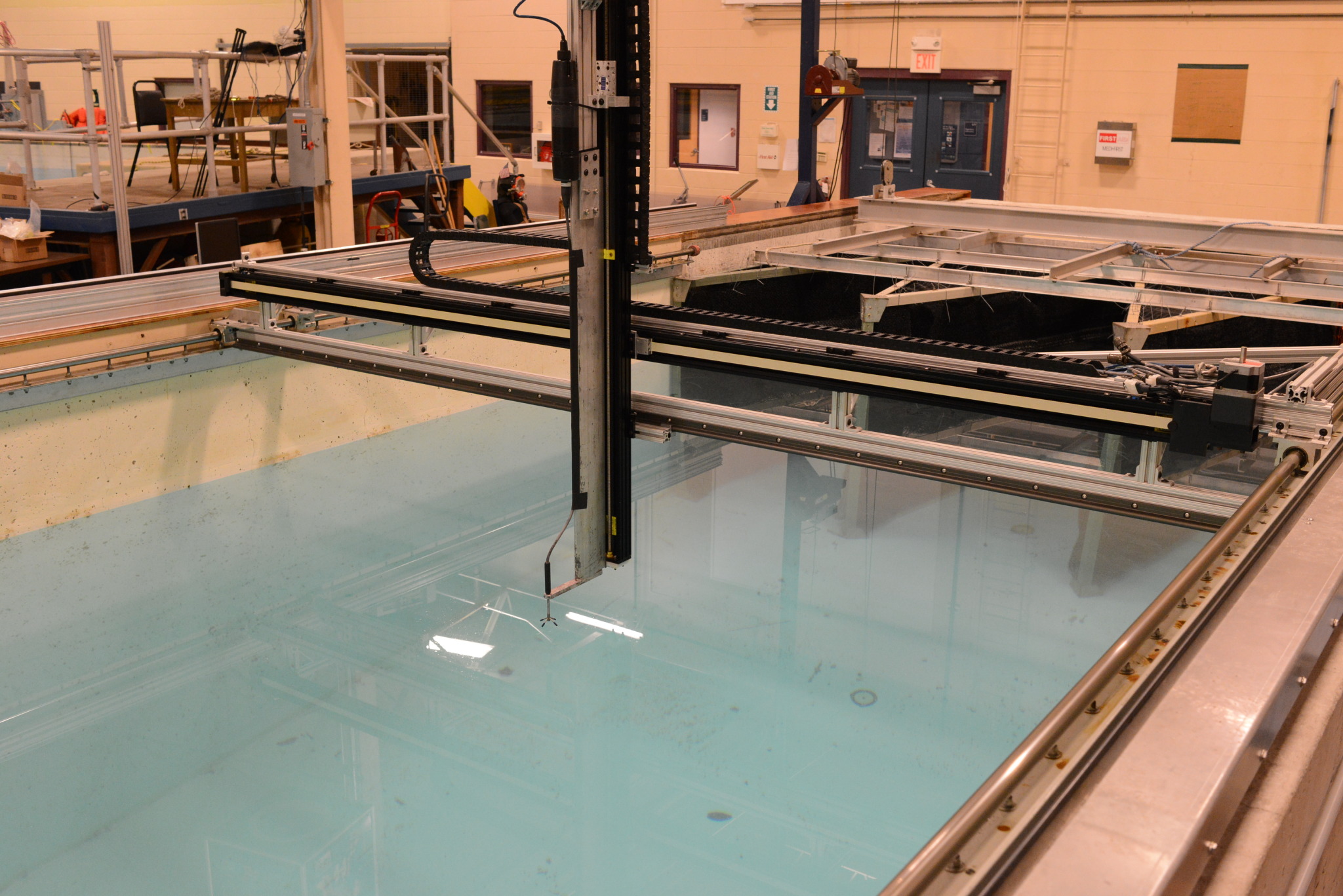
Wake measurement instrumentation

• Nortek Vectrino+ acoustic Doppler velocimeter (ADV)
• $y$–$z$ traversing carriage with motion control integration

Automation

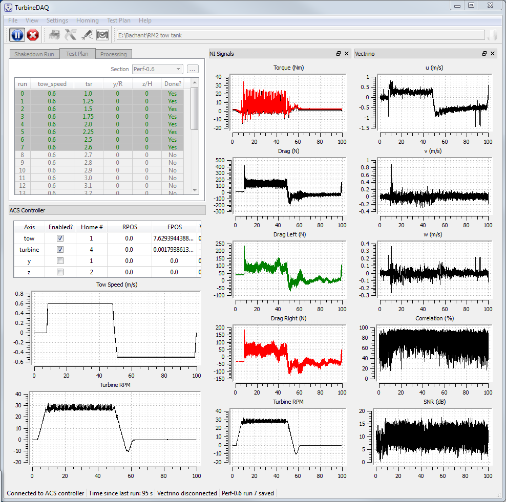
Operation

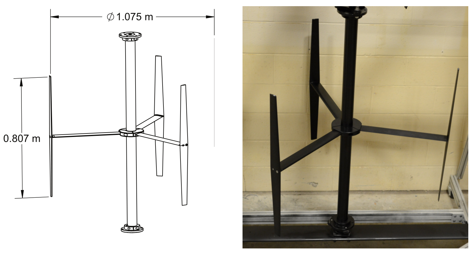
UNH-RVAT baseline experiments

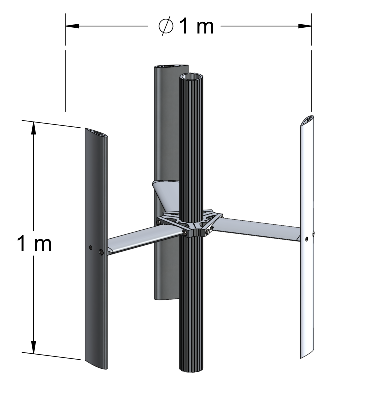
• Simple geometry
• NACA 0020 foils
• High solidity $c/R = 0.28$
• $U_\infty = 1$ m/s
• Characterize performance
• Near-wake dynamics
• Open dataset

Bachant, P., and Wosnik, M. (2015) "Characterising the near-wake of a cross-flow turbine", Journal of Turbulence, 16, 392–410.

Bachant, P., and Wosnik, M. (2014) "UNH-RVAT baseline performance and near-wake measurements: Reduced dataset and processing code", Figshare, DOI: 10.6084/m9.figshare.1080781.

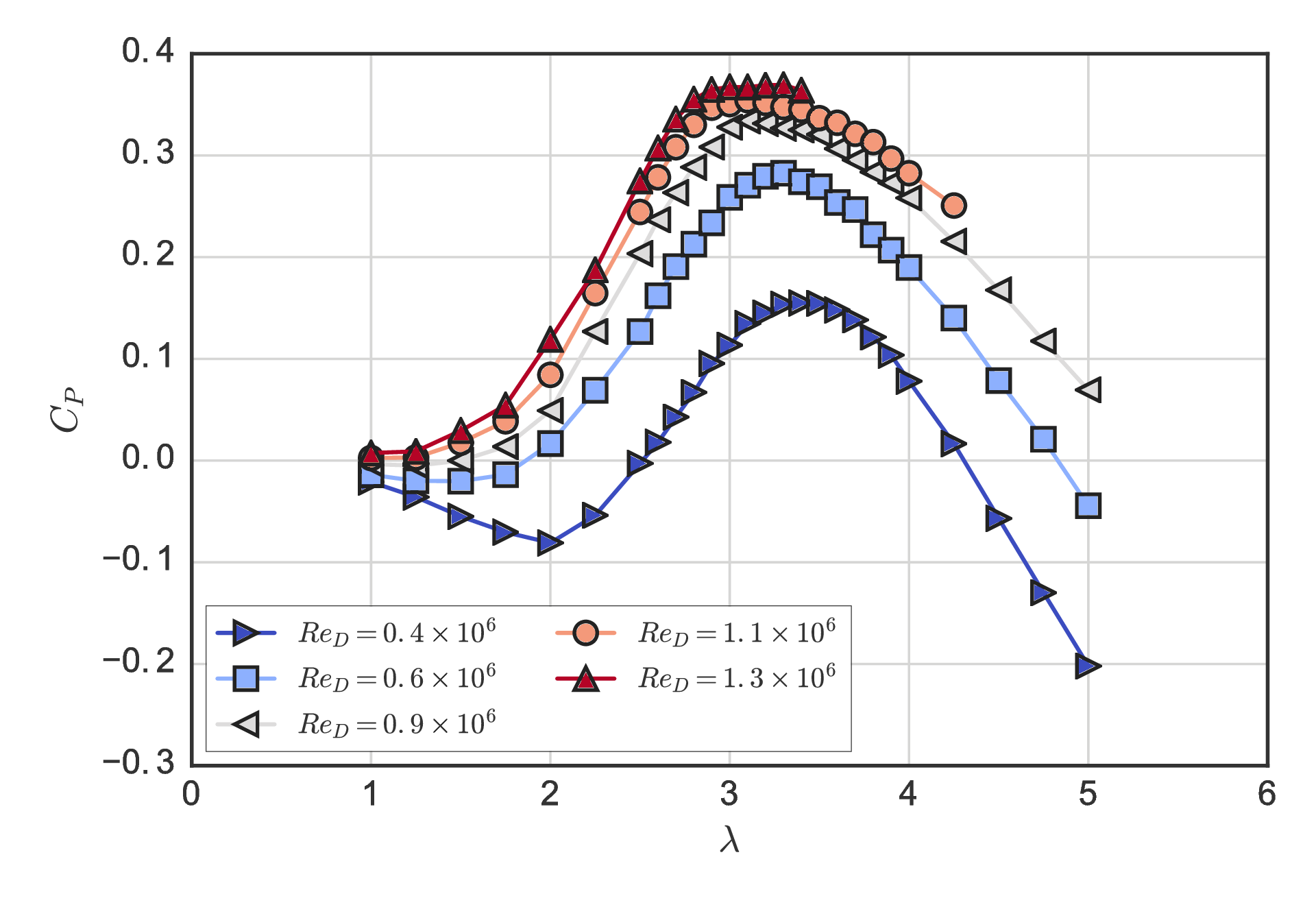
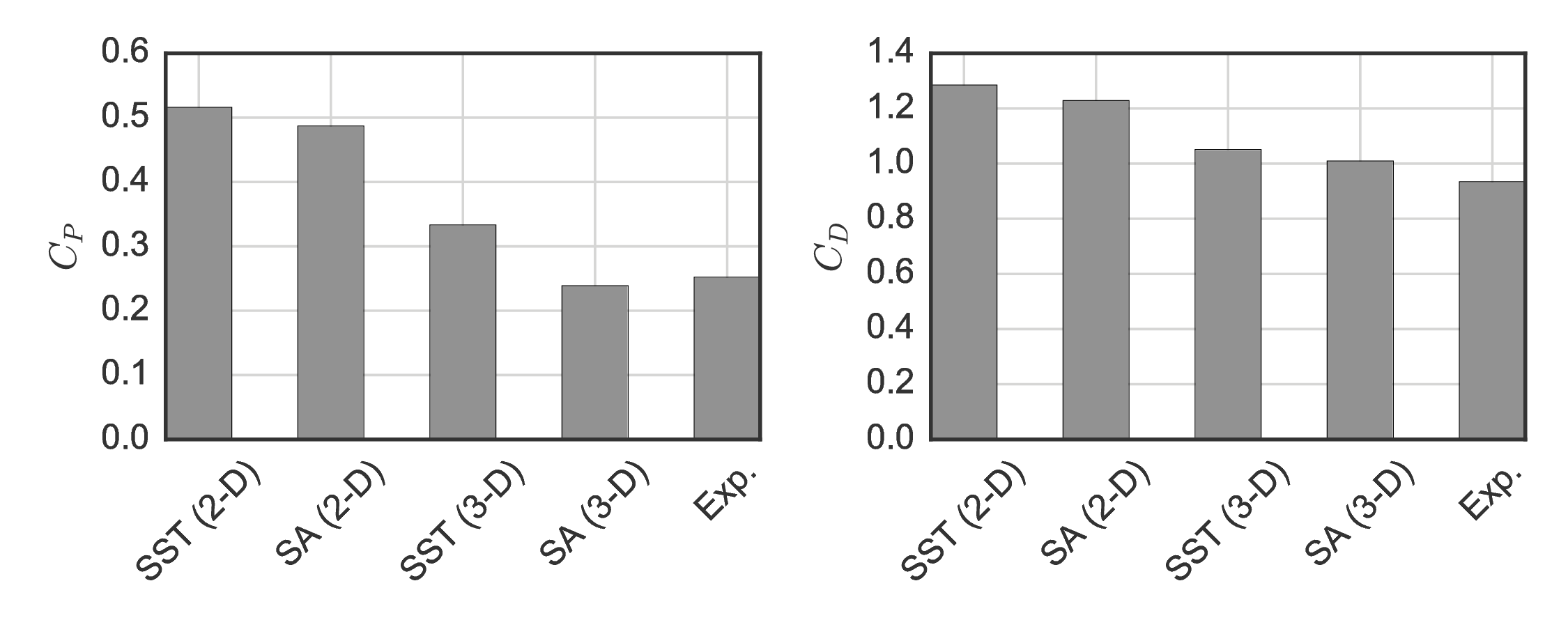
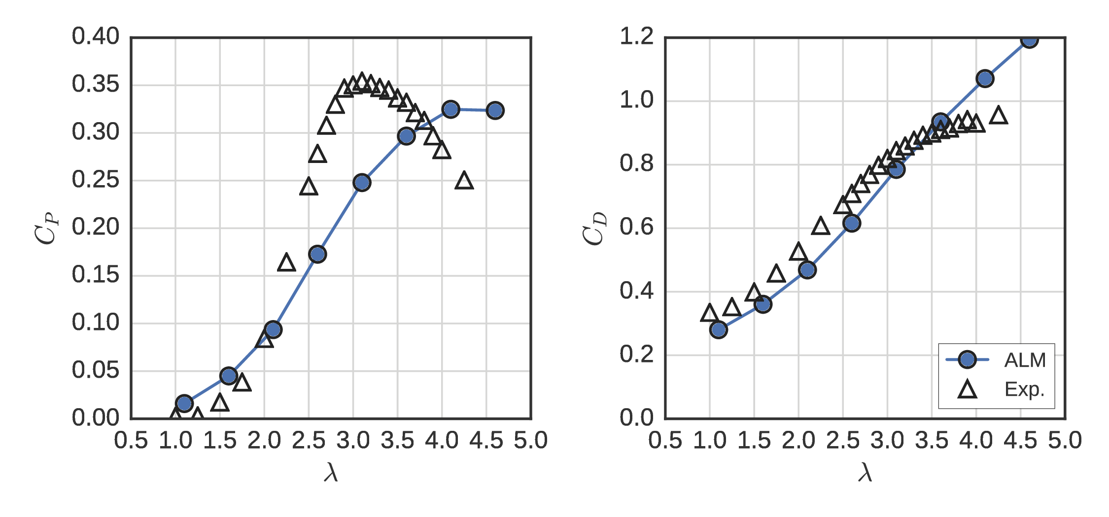
UNH-RVAT baseline performance

# Generate figures from the experiments by their own methods

os.chdir("C:/Users/Pete/Research/Experiments/RVAT baseline")
import pyrvatbl.plotting as rvat_baseline

fig, (ax1, ax2) = plt.subplots(figsize=(15, 6), nrows=1, ncols=2)
rvat_baseline.plot_cp(ax1)
rvat_baseline.plot_cd(ax2, color=sns.color_palette()[2])
fig.tight_layout()
os.chdir(talk_dir)

$\lambda = \frac{\omega R}{U_\infty}$         $C_P = \frac{P_\mathrm{mech}}{\frac{1}{2}\rho A_\mathrm{f} U_\infty^3}$         $C_D = \frac{F_\mathrm{drag}}{\frac{1}{2}\rho A_\mathrm{f} U_\infty^2}$

Note: Overall rotor drag (sometimes called thrust) coefficient $C_D$ is different from blade element drag coefficient $C_d$.

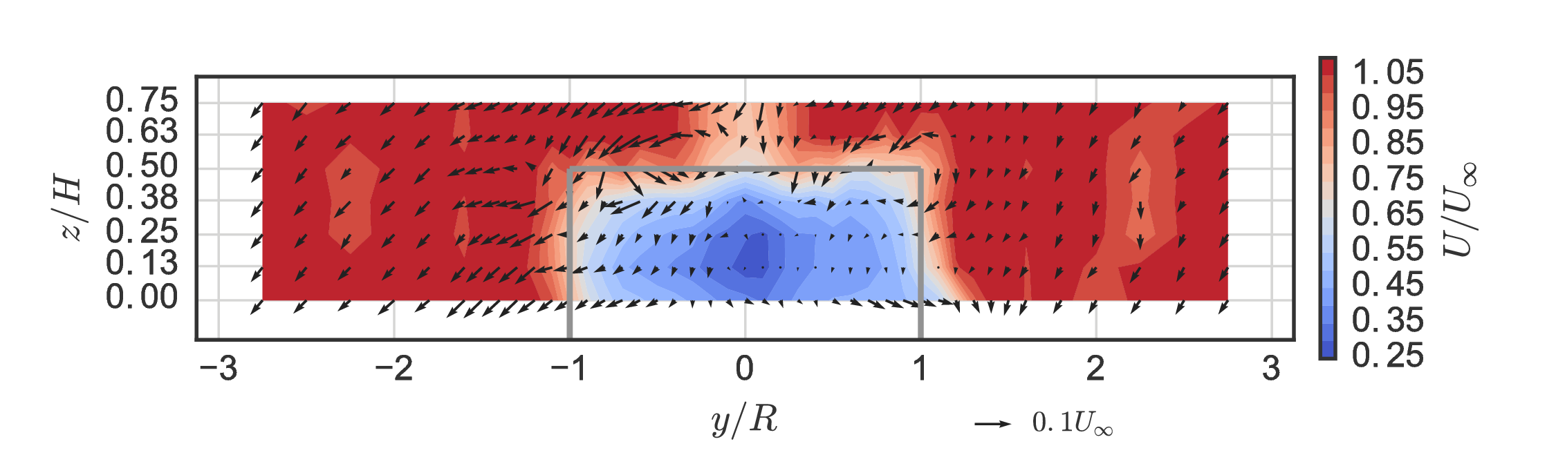
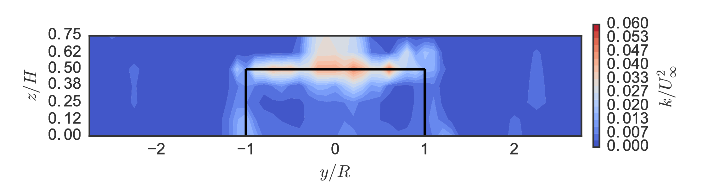
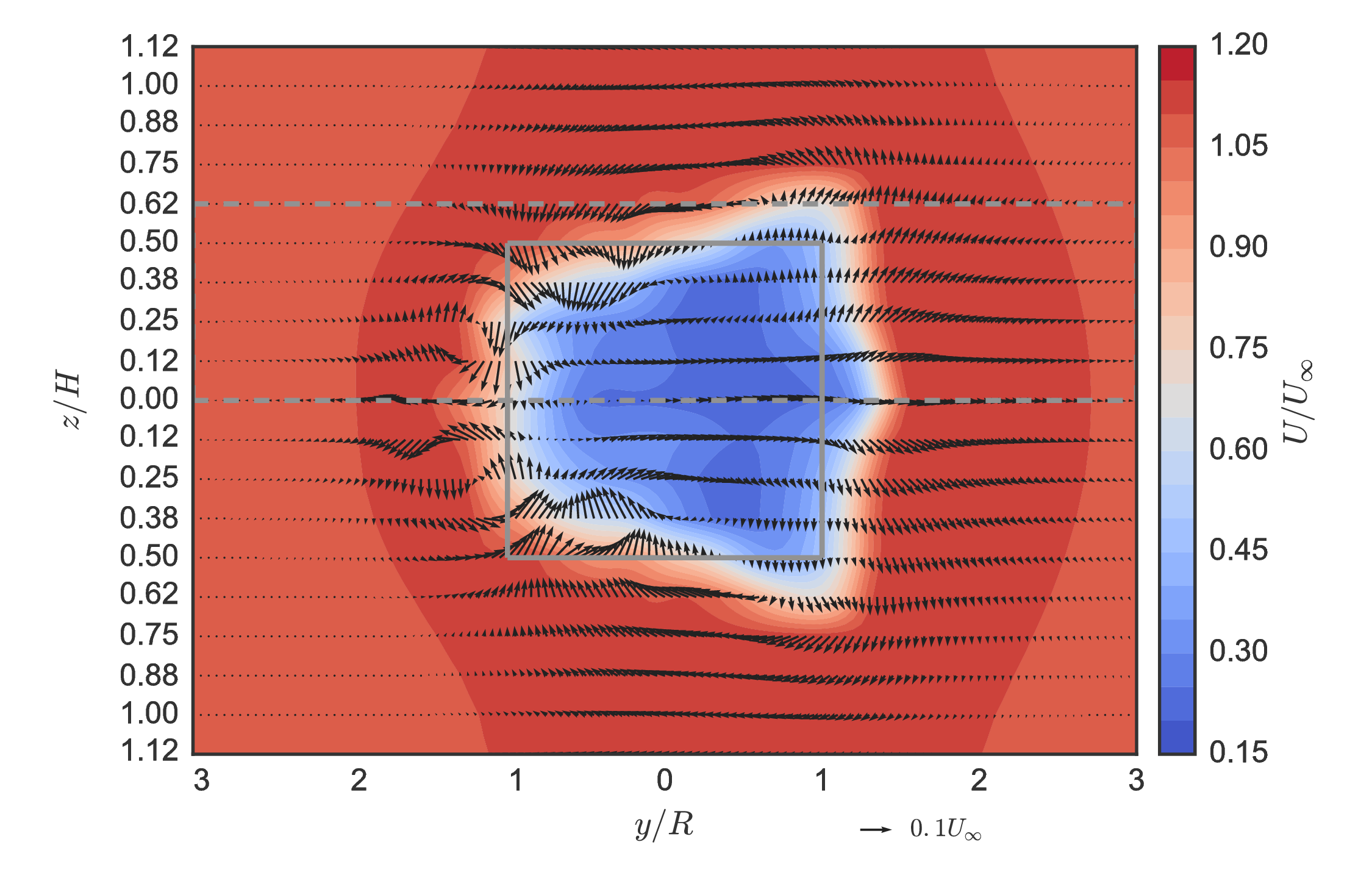
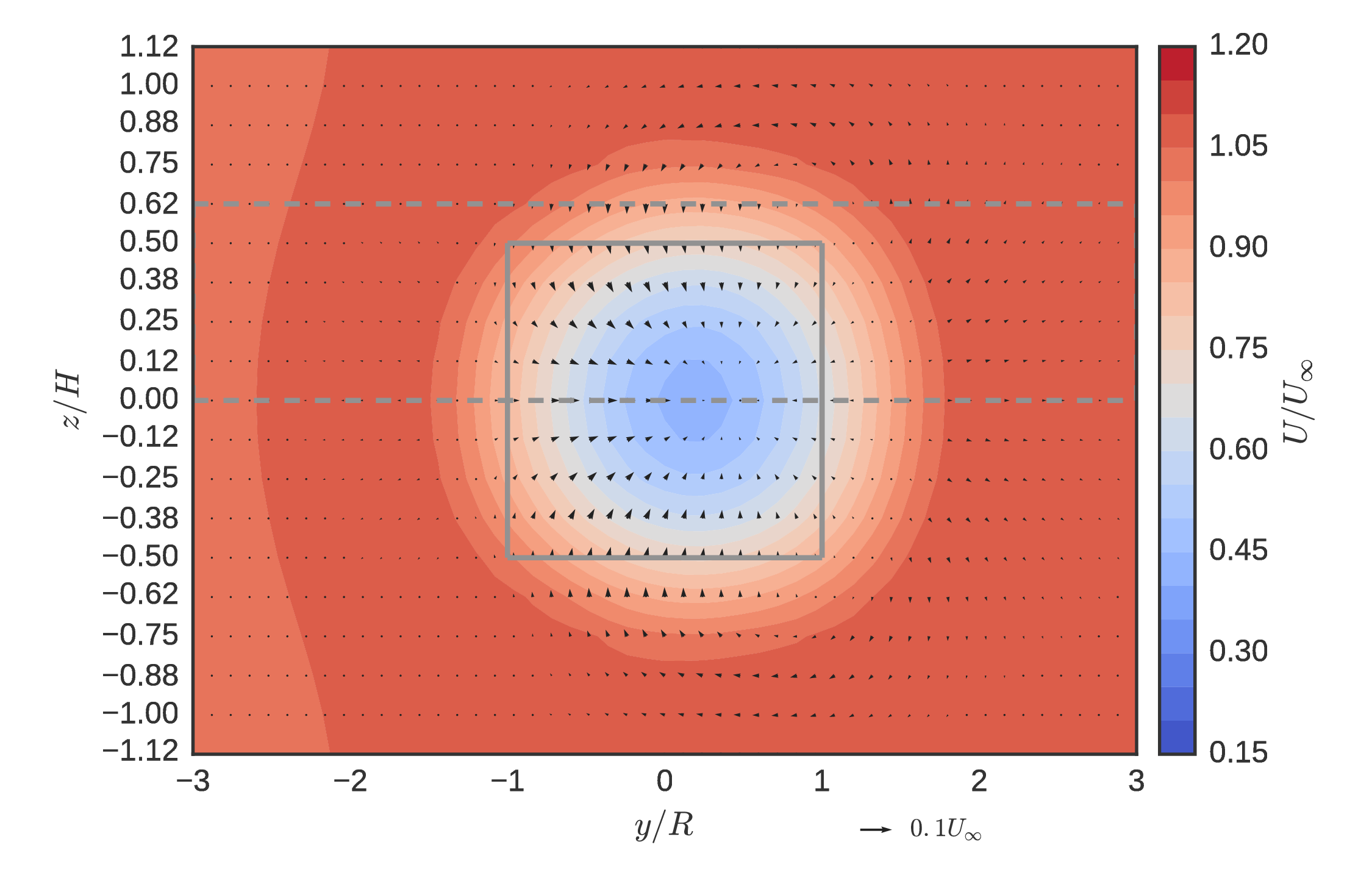
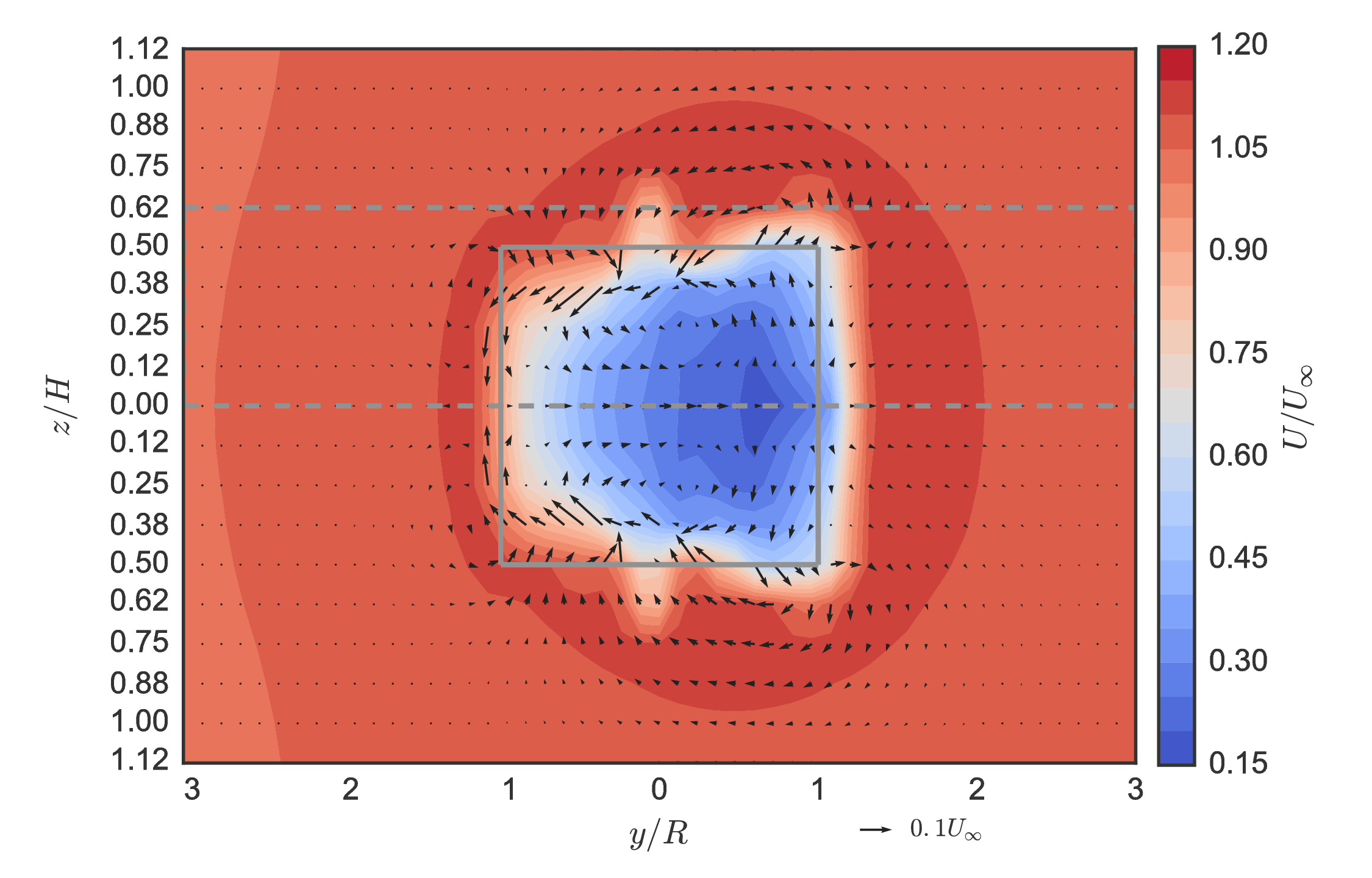
Baseline wake measurements $(x/D=1)$

UNH-RVAT baseline wake characteristics

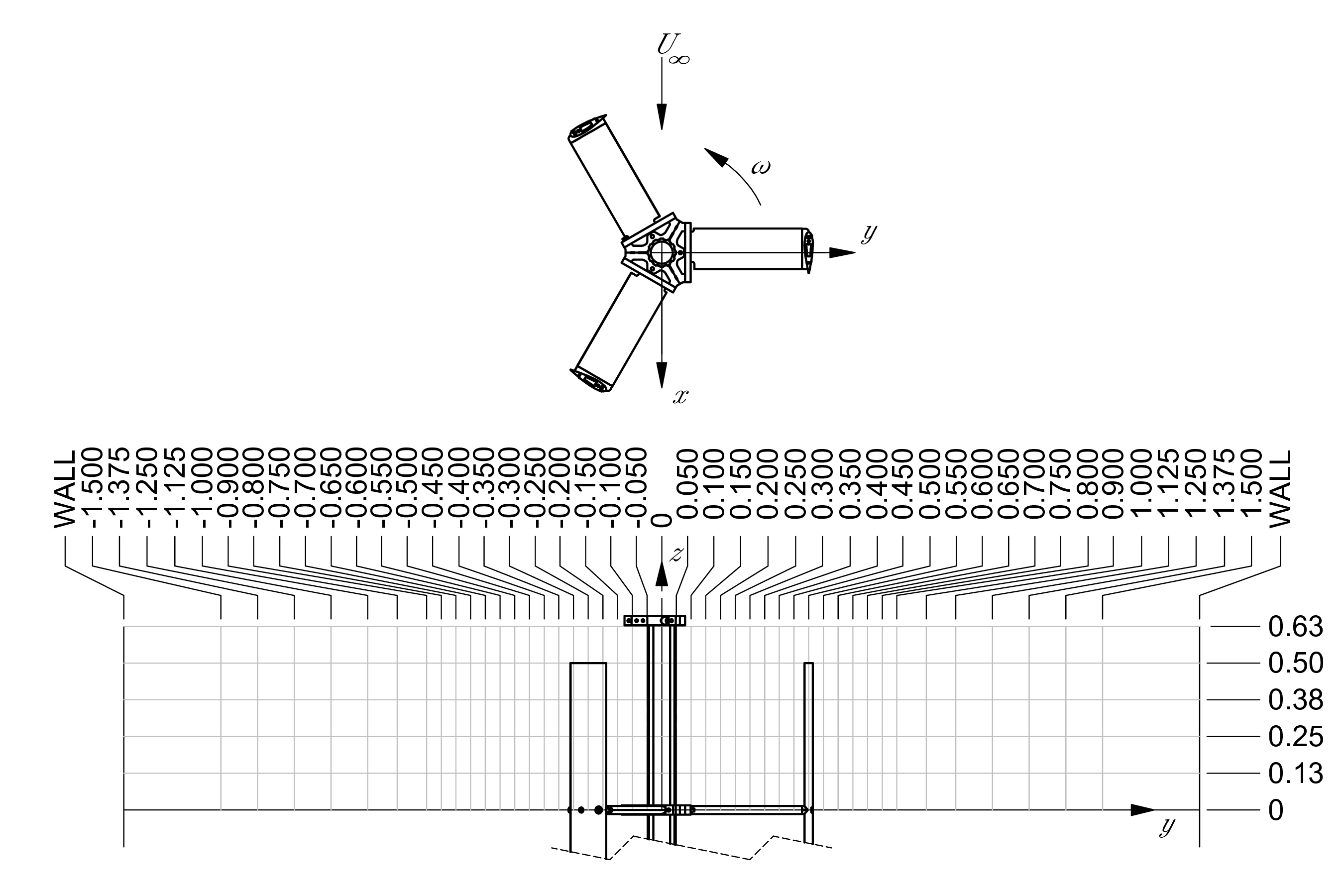
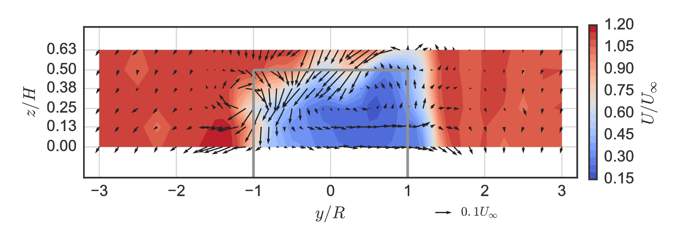
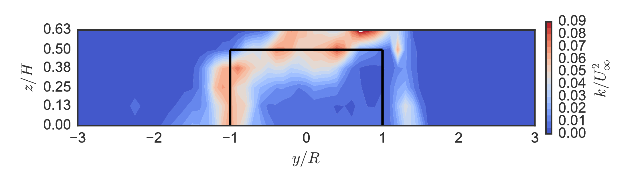
Unique mean "doublet" flow created by blade tip vortices inducing vertical velocity towards $x$–$y$ center plane.

One might guess this mean vertical velocity is important, since for an AFT you have a uniform swirl, but we want to compare to the turbulence.

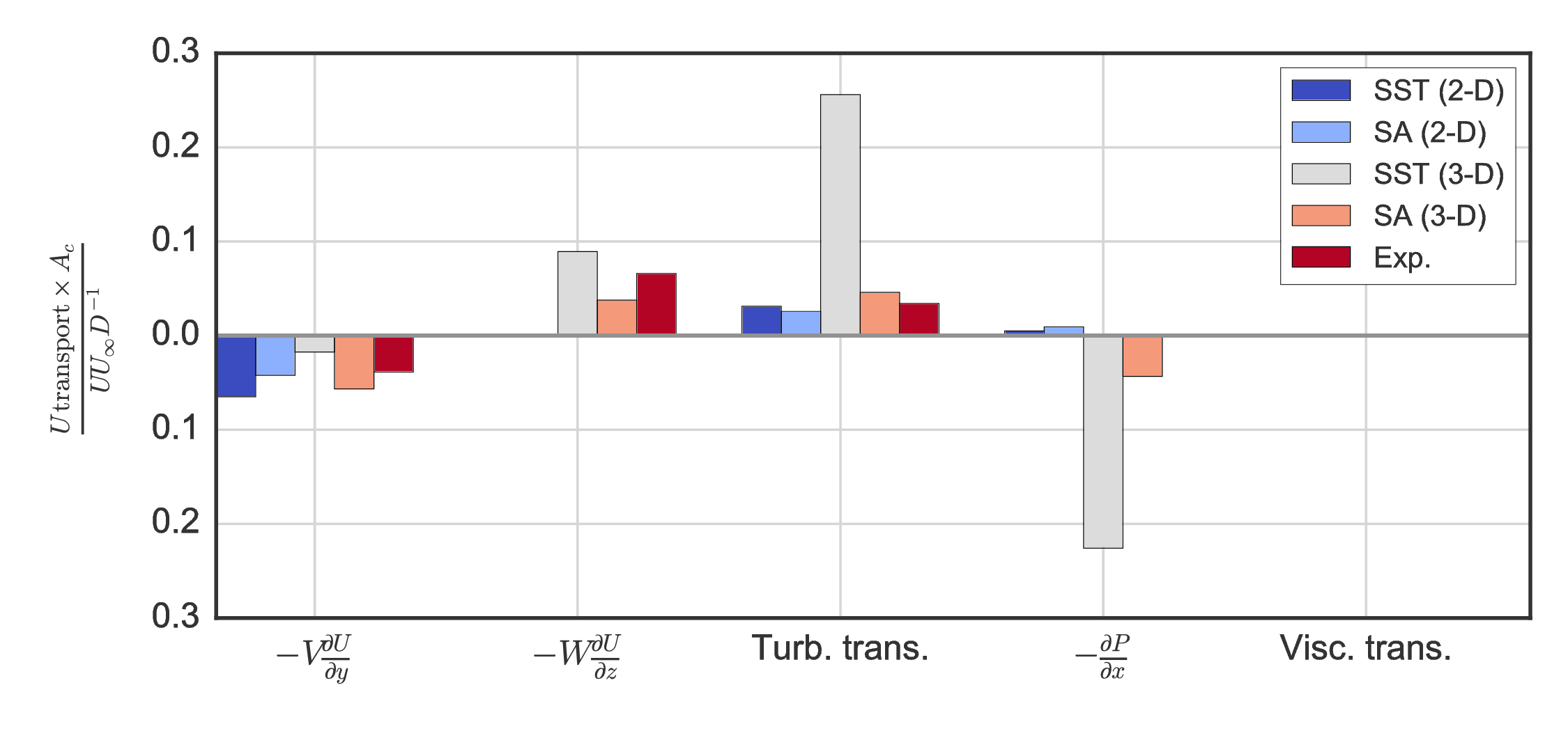
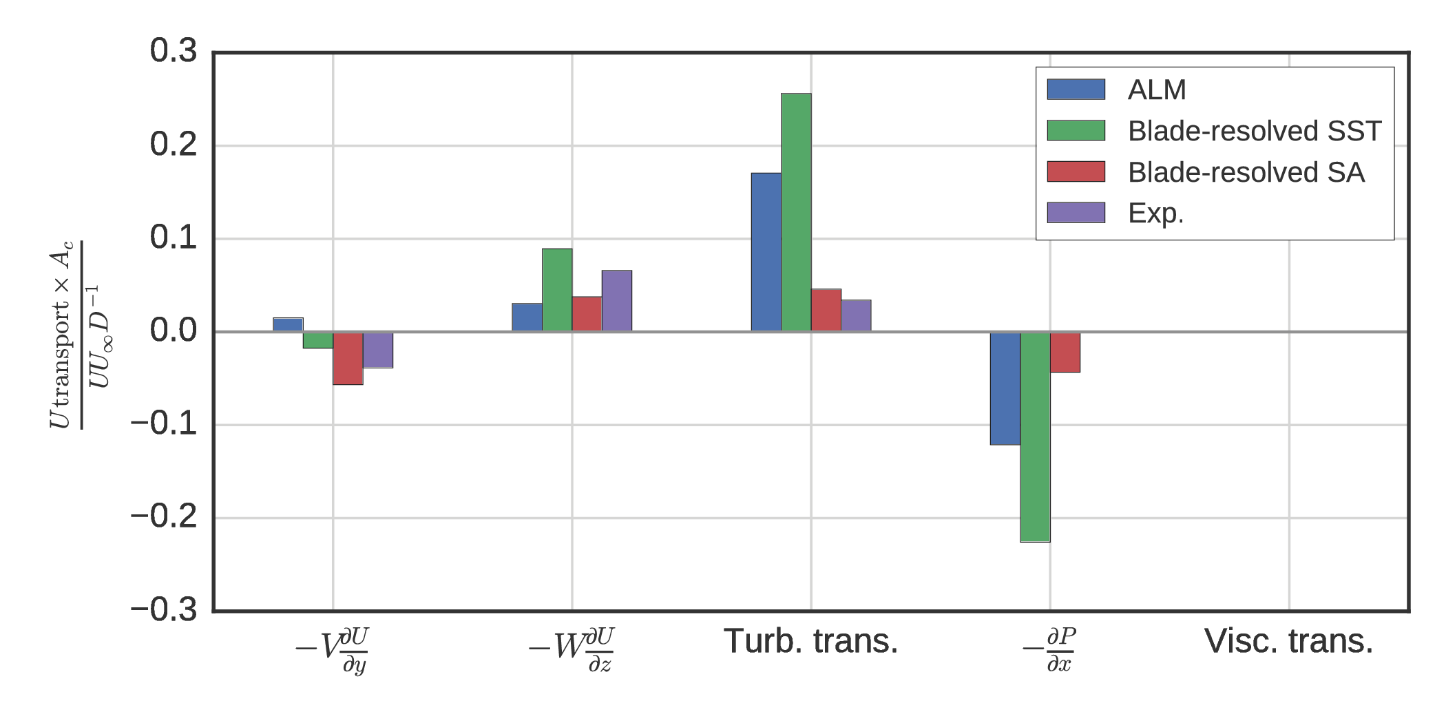
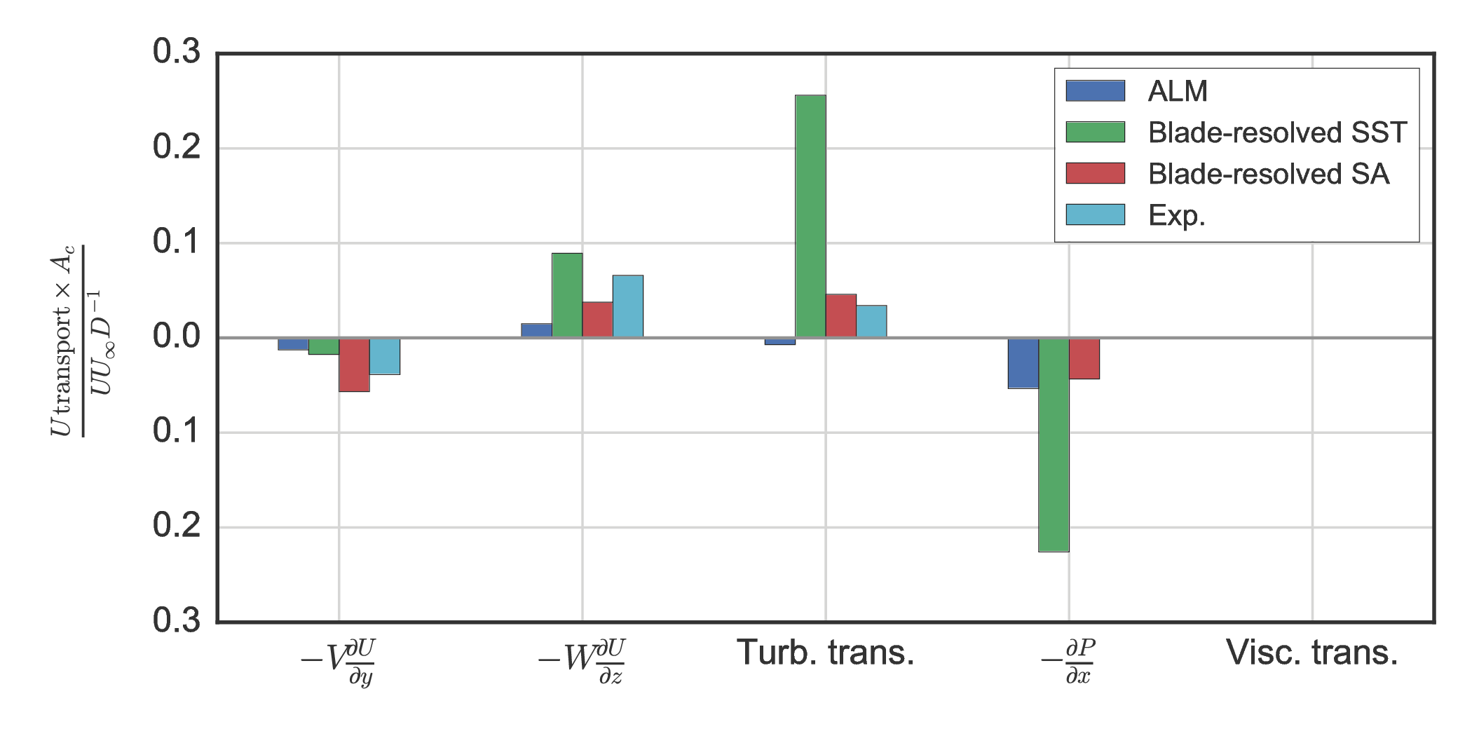
Mean momentum transport

Rearrange RANS to isolate streamwise partial derivative:

$$ \begin{split} \frac{\partial U}{\partial x} = \frac{1}{U} \bigg{[} & - V\frac{\partial U}{\partial y} - W\frac{\partial U}{\partial z} \\ & -\frac{1}{\rho}\frac{\partial P}{\partial x} \\ & - \frac{\partial}{\partial x} \overline{u'u'} - \frac{\partial}{\partial y} \overline{u'v'} - \frac{\partial}{\partial z} \overline{u'w'} \\ & + \nu\left(\frac{\partial^2 U}{\partial x^2} + \frac{\partial^2 U}{\partial y^2} + \frac{\partial^2 U}{\partial z^2} \right) \bigg{]} \end{split} $$

Mean momentum transport

Weighted averages at $x/D=1$:

os.chdir("C:/Users/Pete/Research/Experiments/RVAT baseline")
import pyrvatbl.plotting as rvat_baseline

rvat_baseline.plotwake("mombargraph", scale=1.8, barcolor=None)
plt.grid(True)

Mean advection in AFT wake due to axisymmetric swirl would cancel itself out.

UNH-RVAT Reynolds number dependence

Are our results relevant to full scale?

$$ Re_l = \frac{Ul}{\nu} $$

How inexpensive (small, slow) can experiments get?

Bachant, P., and Wosnik, M. (2016) "Effects of Reynolds Number on the Energy Conversion and Near-Wake Dynamics of a High Solidity Vertical-Axis Cross-Flow Turbine", Energies, 9.

Bachant, P., and Wosnik, M. (2016) "UNH-RVAT Reynolds number dependence experiment: Reduced dataset and processing code", Figshare, DOI: 10.6084/m9.figshare.1286960.

UNH-RVAT Reynolds number dependence

os.chdir(rvat_re_dep_dir)
import pyrvatrd.plotting as rvat_re_dep

fig, (ax1, ax2) = plt.subplots(figsize=(16, 6.5), nrows=1, ncols=2)
rvat_re_dep.plot_perf_curves(ax1, ax2)
fig.tight_layout()
os.chdir(talk_dir)

Note effects of stall delay at lower $\lambda$, where angle of attack amplitude is greater.

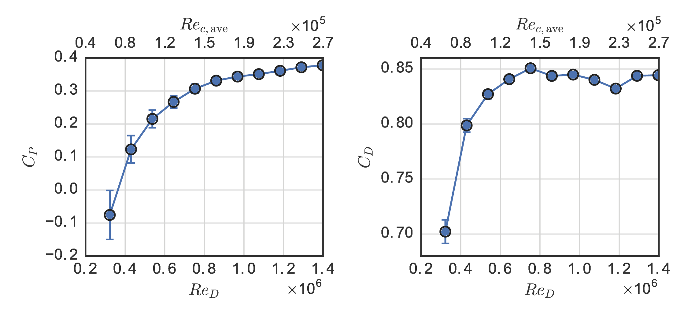
Reynolds number dependence at $\lambda = 1.9$

os.chdir(rvat_re_dep_dir)
import pyrvatrd.plotting as rvat_re_dep

fontsize = plt.rcParams["font.size"]

with plt.rc_context({"axes.formatter.use_mathtext": True, "font.size": fontsize*1.65/1.5}):
    fig, (ax1, ax2) = plt.subplots(figsize=(14, 6), nrows=1, ncols=2)
    rvat_re_dep.plot_perf_re_dep(ax1, ax2, errorbars=True, label_subplots=False)
    fig.tight_layout()
    
os.chdir(talk_dir)

$$ Re_{c,\mathrm{ave}} = \lambda U_\infty c / \nu $$

Threshold corresponds to blade boundary layer transition to turbulence, which delays separation to higher angles of attack.

$$ Fr = \frac{U_\infty}{\sqrt{gh_{\mathrm{tip}}}} = 0.1 \text{ to } 0.5 $$

Wake transport totals

os.chdir(rvat_re_dep_dir)
import pyrvatrd.plotting as rvat_re_dep

fig, ax = plt.subplots()
with plt.rc_context({"axes.formatter.use_mathtext": True}):
    rvat_re_dep.plot_wake_trans_totals(ax)
fig.tight_layout()

Similar threshold $Re$ as for $C_P$ → Low $Re$ physical model array studies may overpredict power of downstream turbines

DOE/SNL Reference Model 2 (RM2) experiments

DOE Reference Models: Open designs for standardized development and validation

Measured performance, $Re$-dependence, near-wake, strut drag, with 1:6 scale tapered-H rotor: NACA 0021 profiles, $c/R = 0.07$–$0.12$

Unique geometry for testing predictive robustness

Bachant, P., Gunawan, B., Wosnik, M., and Neary, V.S. (2016) "UNH RM2 tow tank experiment: Reduced dataset and processing code", Figshare, DOI: 10.6084/m9.figshare.1373899.

• Give background on RM2 project
• State blade profile

RM2 performance curves

Higher peak $C_P = 0.37$ vs. UNH-RVAT's $0.26$.

RM2 performance $Re$-dependence at $\lambda = 3.1$

Retains weak $Re$-dependence → lower $c/R$ or virtual camber

RM2 near-wake

$Re_D = 1.1 \times 10^6$, $x/D=0.93$, $\lambda=3.1$

Similar wake recovery proportions, but lower overall compared to UNH-RVAT → potential trade-off vs. higher $C_P$

UNH-RVAT blade-resolved RANS

• Simulate baseline with OpenFOAM

• Need to resolve the boundary layer
• Separation
• Transition?
• Turbulence models (eddy viscosity)
• $k$–$\omega$ SST
• Spalart–Allmaras
• 2-D: $\sim 0.1$ CPU hours per simulated second
• 3-D: $\sim 10^3$ CPU hours per simulated second
• HPC required: significant investment
• 192 cores on SNL Red Mesa cluster

Cluster may cost about the same as a physical model experiment!

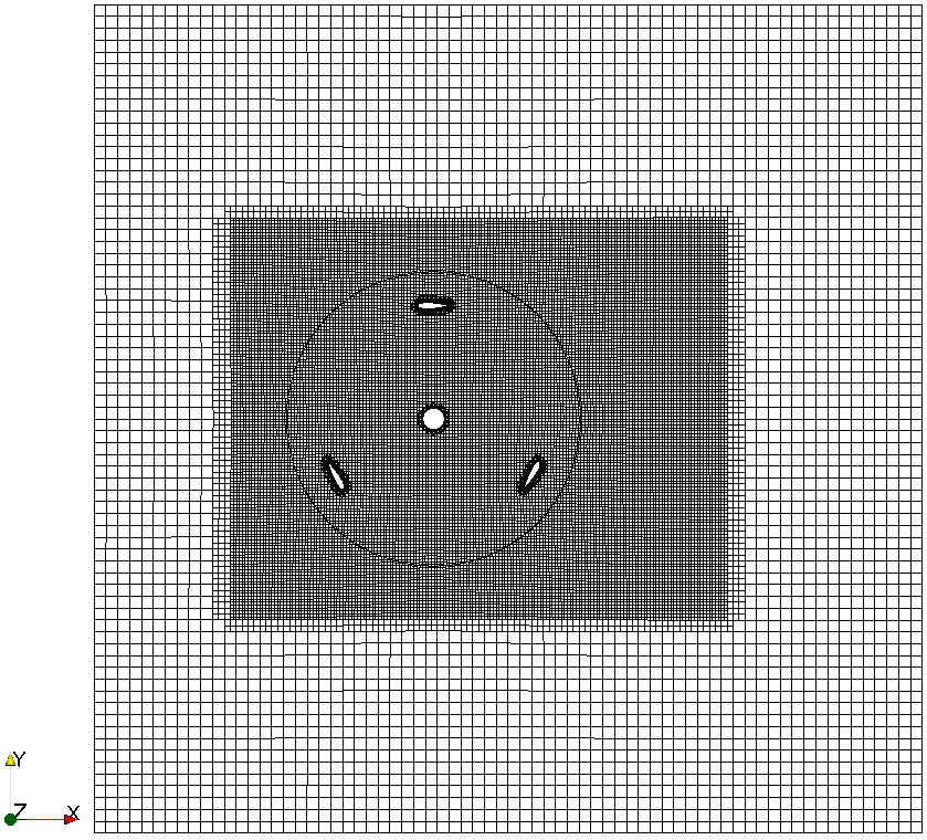
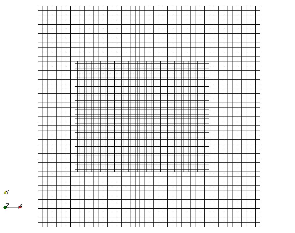
Mesh topology overview

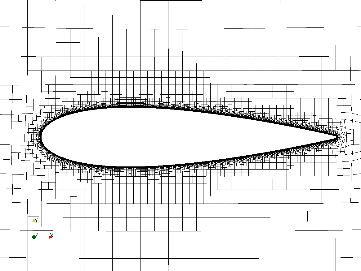
Near-wall blade mesh

$$ y^+ = u^* y / \nu \sim 1 $$$$ u^*=\sqrt{\tau_w / \rho} $$

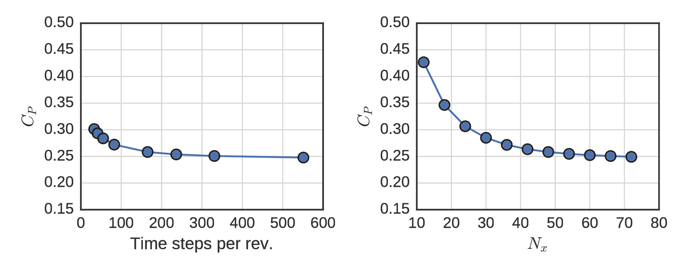
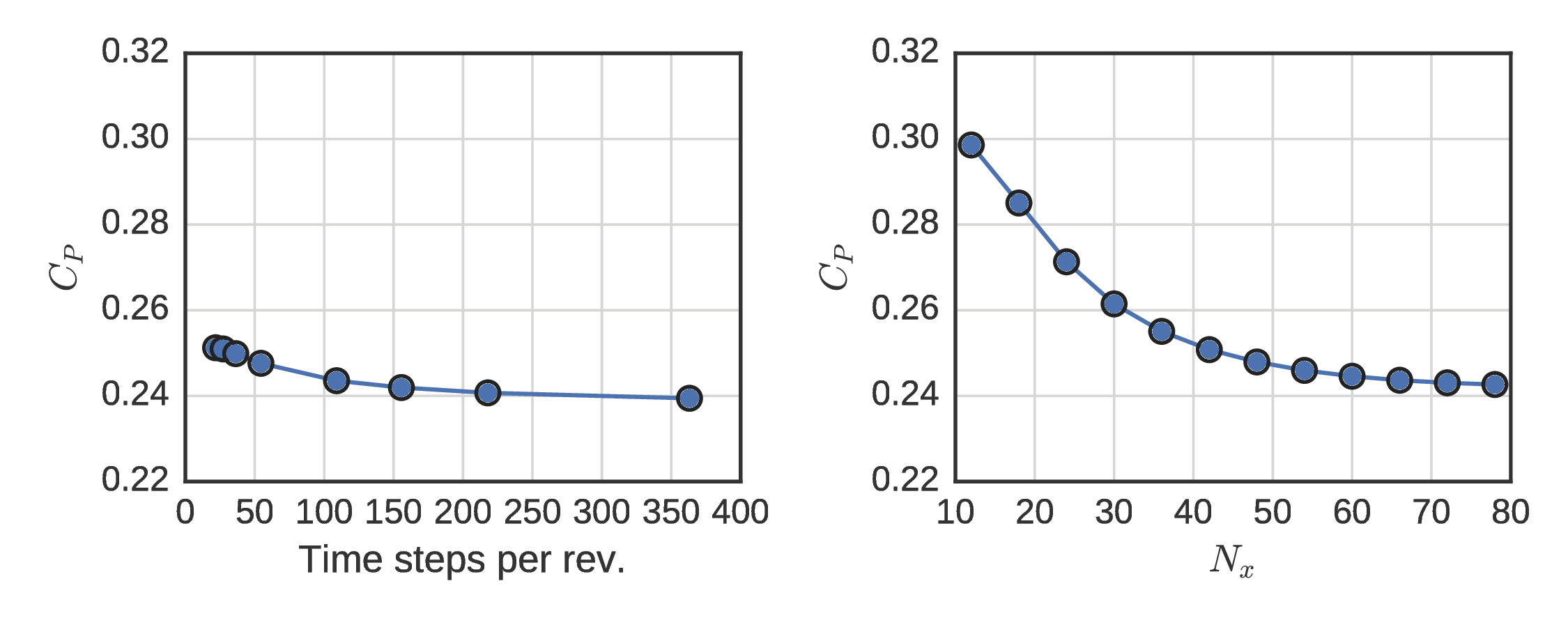
Verification (2-D)

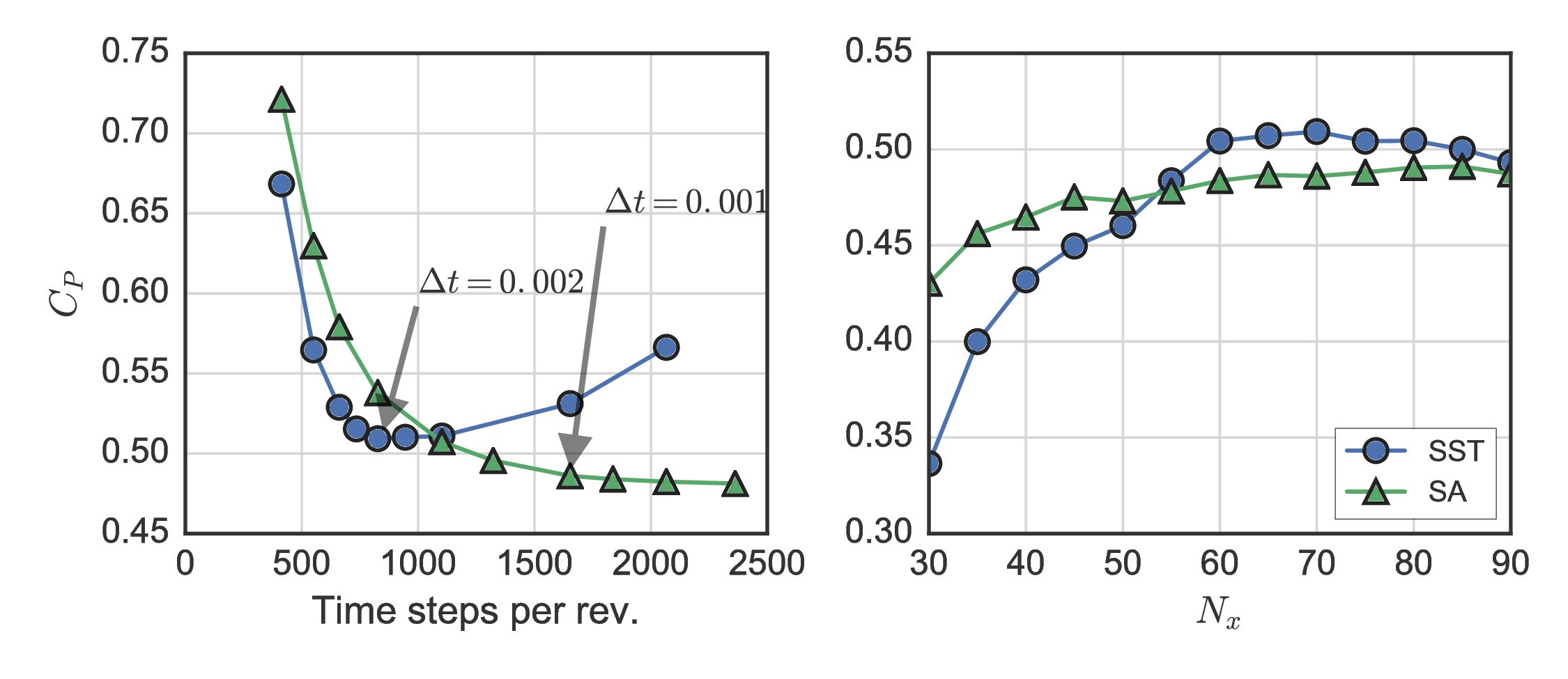
Spalart–Allmaras model showed more well-behaved grid convergence. Relative minimum chosen for SST $\Delta t$. $N_x = 70$ chosen for both models.

Performance predictions

Overprediction by 2-D simulations consistent with the literature.

Near-wake mean velocity

3-D Spalart–Allmaras

Experiment

Near-wake mean velocity

3-D SST

Experiment

Near-wake momentum transport

Weighted sums for CFD computed over entire domain at $x/D=1$

Actuator line modeling

• Developed by Sorensen and Shen (2002)
• Blade element method coupled with Navier–Stokes
• Save computational resources
  • No finely resolved blade boundary layers
  • No complicated meshing
  • No mesh motion
• Current state-of-the-art for HAWT array modeling
• Has only been investigated with LES for a 2-D low-$Re$ CFT by Shamsoddin and Porte-Agel (2014)
  • No performance predictions reported
  • Closed source

ALM blade element discretization

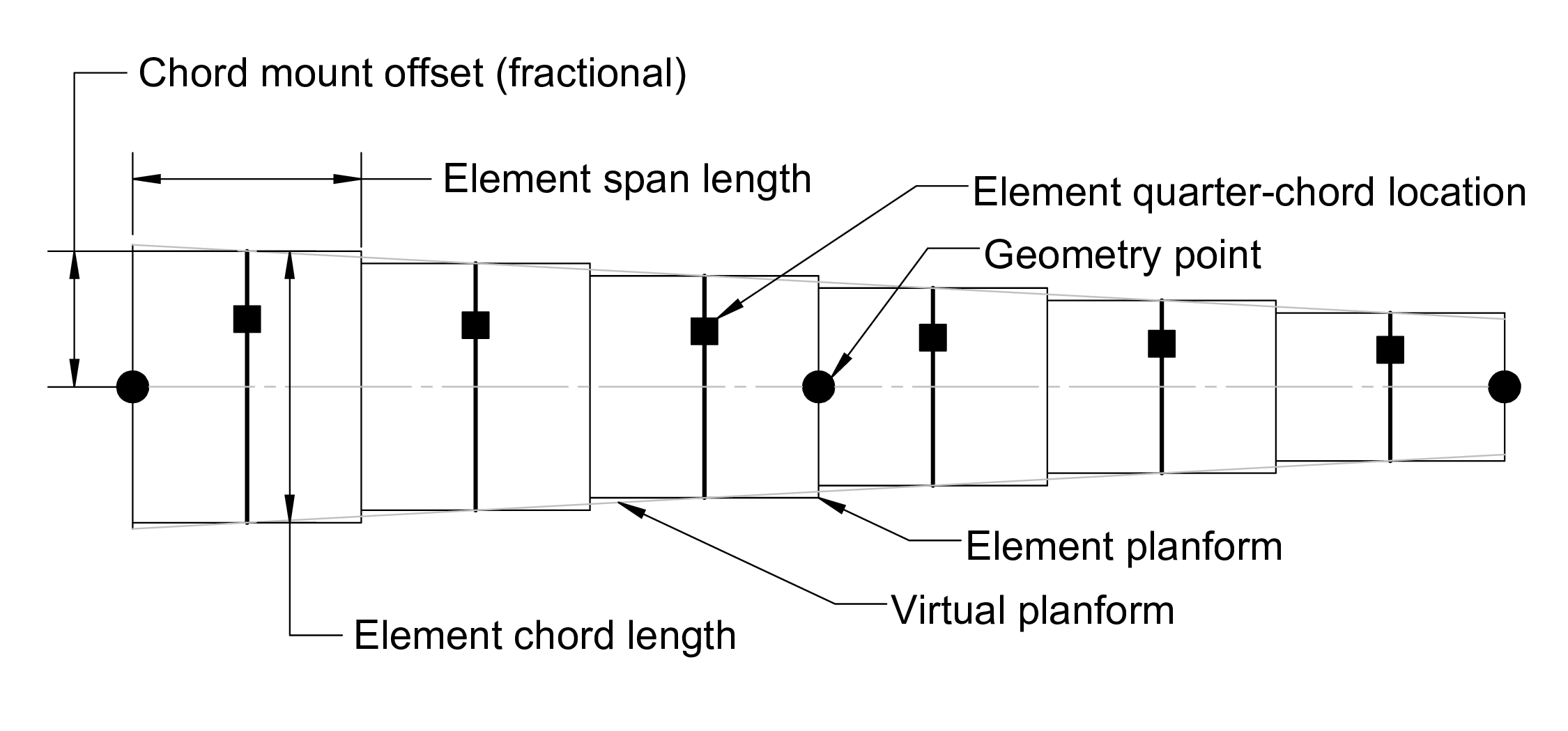
Computing blade loading

Inflow velocity from Navier–Stokes solver rather than via simple momentum, potential flow (vortex method).

$$ F_l = \frac{1}{2} \rho A_p C_l | U_{\mathrm{rel}} |^2 \, \, \, \, \, \, \, \, \, F_d = \frac{1}{2} \rho A_p C_d | U_{\mathrm{rel}} |^2 $$

import warnings
warnings.filterwarnings("ignore")
os.chdir(os.path.join(os.path.expanduser("~"), "Google Drive", "Research", "CFT-vectors"))
import cft_vectors
fig, ax = plt.subplots(figsize=(13, 13))
fontsize = plt.rcParams["font.size"]
with plt.rc_context({"font.size": 1.4*fontsize}):
    cft_vectors.plot_diagram(fig, ax, theta_deg=52, axis="off", label=True)
os.chdir(talk_dir)

Dynamic stall modeling

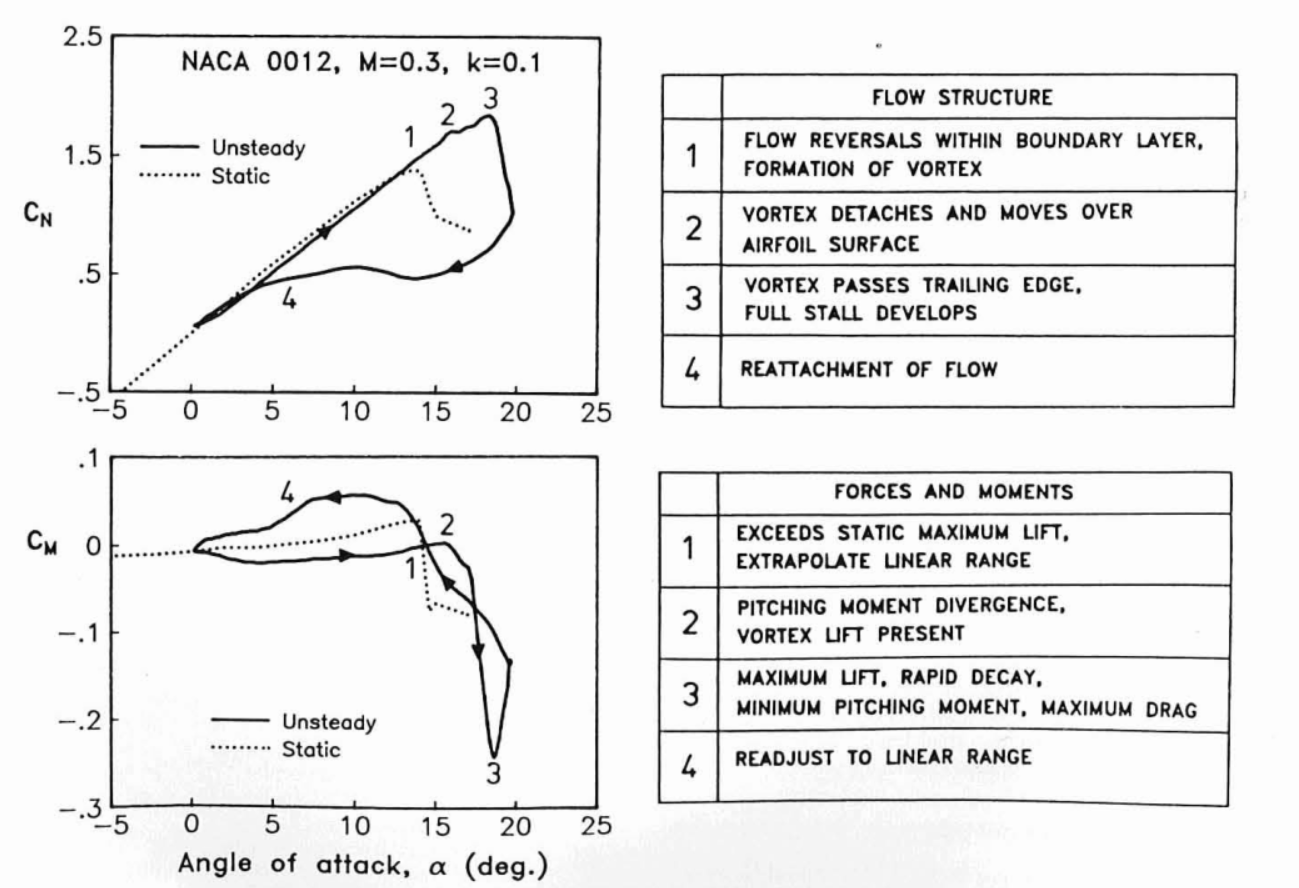
From Leishman and Beddoes (1989)

Leishman–Beddoes semi-empirical dynamic stall model based on lags to angle of attack, separation point, vortex lift, replicating "hysteresis loop."

Flow field coupling

AL force added to Navier–Stokes as body force source term:

$$ \frac{\partial \vec{u}}{\partial t} + \vec{u} \cdot \nabla \vec{u} = -\frac{1}{\rho}\nabla p + \nabla^2 \vec{u} + \boxed{\vec{f}} $$

Force is smoothed outwards with a spherical Gaussian function:

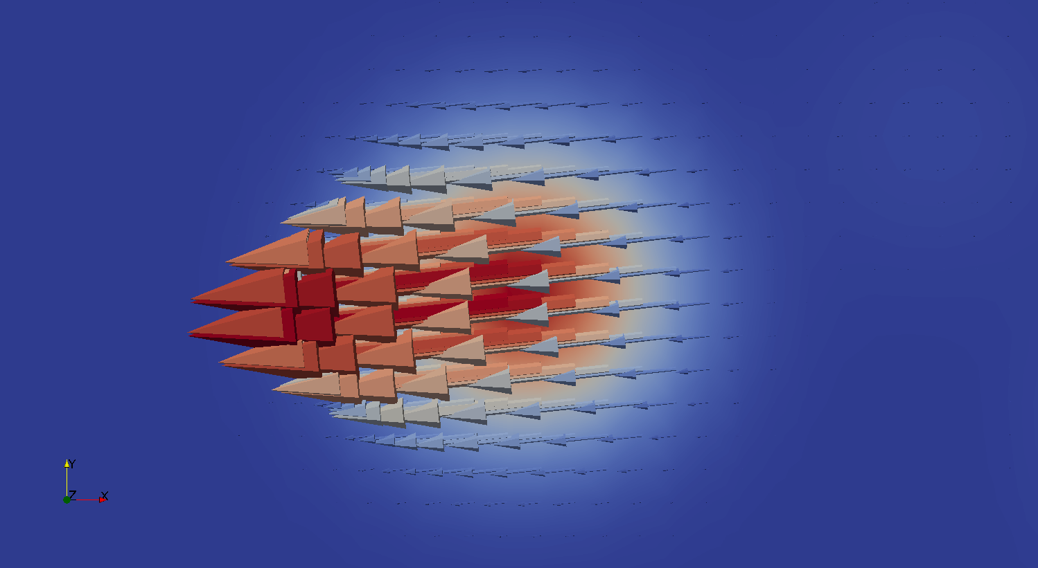
Gaussian width mainly determined by local mesh size: $\approx 2 \Delta x$ (Troldborg, 2008) $\approx 2 \times 2 \sqrt[3] V_{\mathrm{cell}}$

Implementation

OpenFOAM extension library using fvOptions generic mechanism for adding sources at run time:

// Solve the Momentum equation

tmp<fvVectorMatrix> UEqn
(
    fvm::ddt(U)
  + fvm::div(phi, U)
  + turbulence->divDevReff(U)
 ==
    fvOptions(U)
);

Leverage existing solvers, parallelization, turbulence models. No wheel reinvention.

Developed openly on GitHub: https://github.com/turbinesFoam/turbinesFoam

UNH-RVAT and RM2 actuator line simulations

• Leishman–Beddoes DS model modified by Sheng et al. (2008)
• Flow curvature correction from Goude (2012)
• Lifting line based end effects model (not used for RM2)
• Added mass correction from Strickland et al. (1981)
• NACA 0021 static coefficients from Sheldahl and Klimas (1981)
  • Major weakness of BE methods: Need static data, which is surprisingly hard to find
• Standard $k$–$\epsilon$ RANS model (eddy viscosity)

ALM mesh

Similar domain and BCs as 3-D blade-resolved case

$\sim 10^4$ lower computational effort with 3-D RANS compared to blade-resolved → Easily run on laptop

ALM verification

UNH-RVAT

RM2

ALM performance

UNH-RVAT

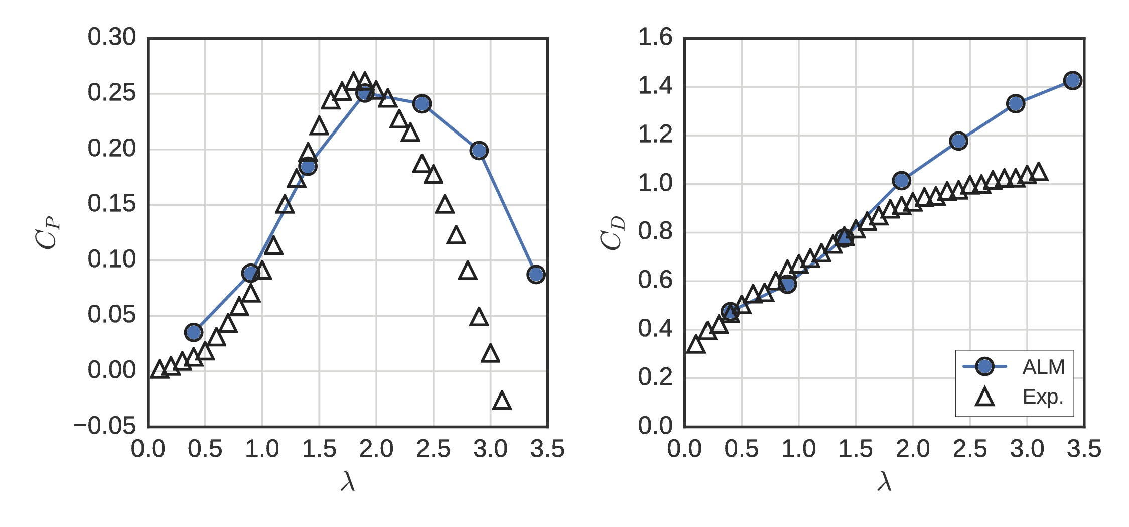
RM2

UNH-RVAT near-wake mean velocity

ALM inside $k$–$\epsilon$ RANS

Low order modeling resolves less detail, but retains asymmetric streamwise deficit, counter-clockwise mean swirl.

UNH-RVAT near-wake momentum transport

ALM inside $k$–$\epsilon$ RANS

Matches trends relatively well except for cross-stream advection

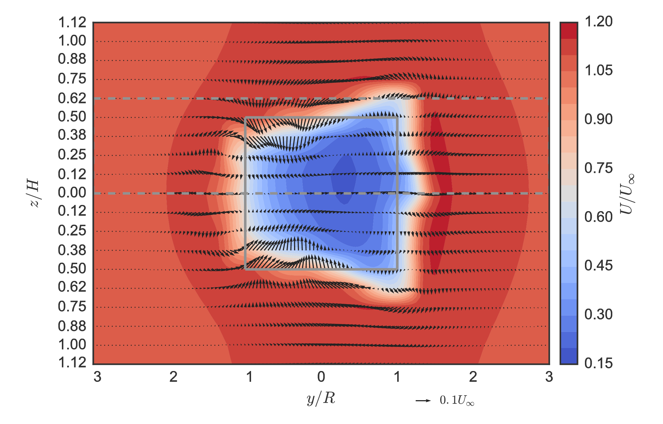
Actuator disk mean velocity at $x/D= 1$

Common streamwise force parameterization based on $C_D$

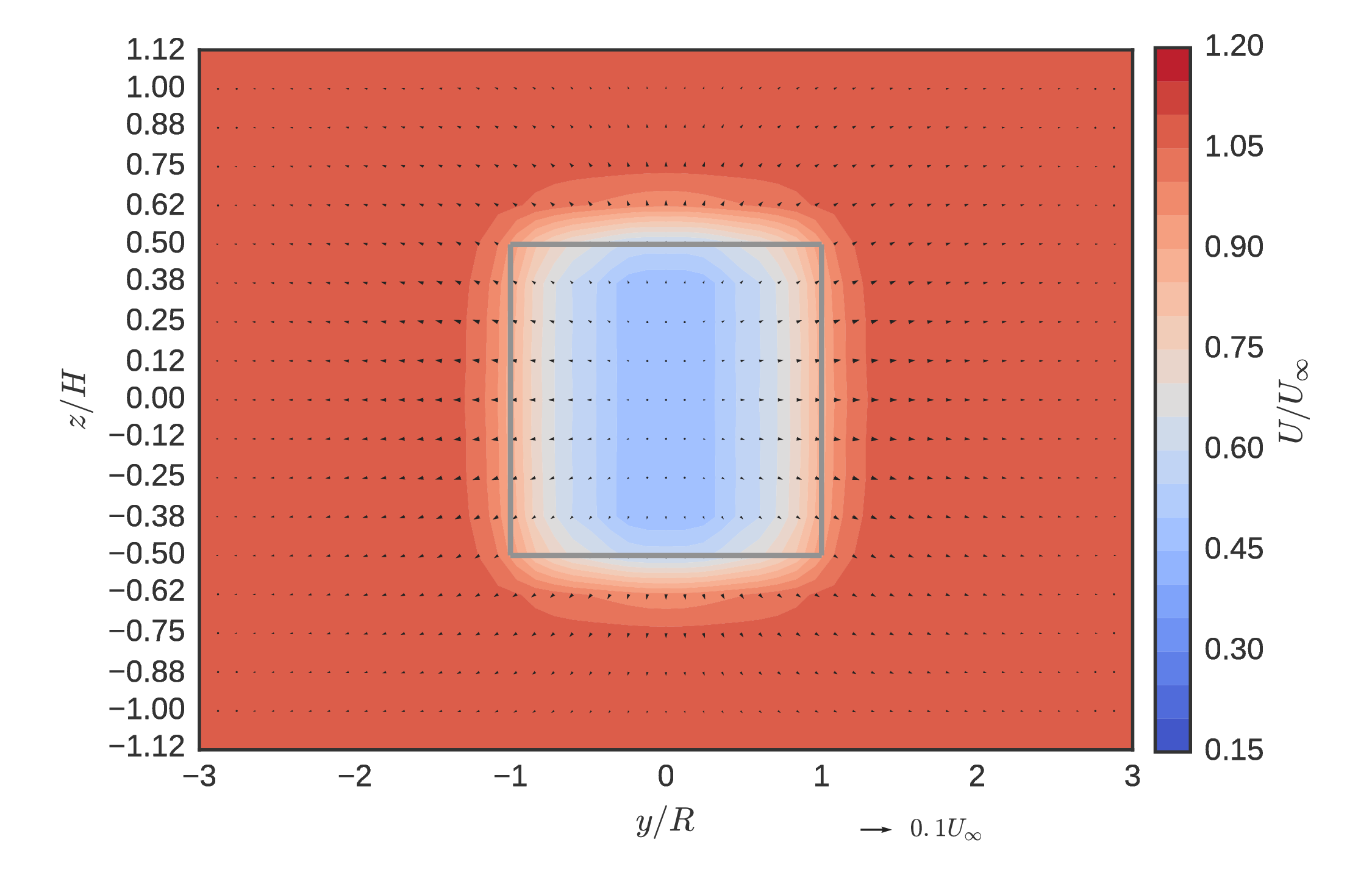
Small negative advection in all directions, very low turbulence, positive pressure gradient effect → ALM generates better IBCs for wake evolution

UNH-RVAT ALM LES

Default Smagorinsky sub-grid scale model

Computational expense up by $\sim 10^2$, still $\sim 10^2$ lower than BR RANS

UNH-RVAT near-wake

ALM inside default Smagorinsky LES

Finer mesh reduces diffusion of counter-clockwise mean swirl

UNH-RVAT near-wake momentum transport

ALM inside default Smagorinsky LES

Small negative turbulence effects → SGS model and vortex breakdown

Conclusions (I)

• Developed an automated turbine test bed and two 1 m scale turbine models
  • High solidity UNH-RVAT and medium/low solidity RM2
• Produced 3 open performance and near-wake datasets
• Near-wake streamwise recovery dominated by vertical advection
• $Re$-independence at $Re_D \sim 10^6$ or $Re_c \sim 10^5$
  • Guidelines for physical model scaling
• Blade-resolved RANS can postdict some results in 3-D
  • Uncertainty w.r.t. turbulence model choice
  • Too expensive for arrays

Conclusions (II)

Developed new open-source ALM library for OpenFOAM

• Fills gap between low- and high-fidelity modeling
• Retains Navier–Stokes description
• Reduce computational effort (not including meshing):

import pandas as pd
data = pd.Series()
data["ALM (3-D LES)"] = 10.0
data["ALM (3-D RANS)"] = 0.1
data["BR CFD (3-D)"] = 10**3
data["BR CFD (2-D)"] = 0.1

with sns.plotting_context(font_scale=3) \
        and plt.rc_context({"axes.formatter.limits": (-1, 1),
                            "axes.formatter.use_mathtext": True}):
    fig, ax = plt.subplots(figsize=(11, 2.5))
    data.plot(ax=ax, kind="barh", logy=False, rot=0)
    ax.set_xlabel("CPU hours per simulated second (approx.)")
plt.show()

• Performance predictions close to 3-D B-R RANS at optimal $\lambda$
• Wake predictions much better than AD, except low turbulent transport in LES
• Promising for future development → Improves with turbulence modeling

• Similar expense as vortex modeling
• Will continue to improve as computing resources and turbulence modeling advance.

Future work

• 2-D blade-resolved RANS for relative optimization
• Investigate wake further downstream
  • Compute streamwise derivatives and overall recovery rate
  • Compare with blade-resolved CFD and ALM
• Vortex breakdown (PIV?) and SGS model selection
• ALM validation against multi-CFT (small array) experiments

Future work: VAT with free surface

Future work: Axial-flow turbine

Extensive AFT validation case by Krogstad and Adaramola (2012)

Acknowledgments